 Wondershare EdrawMind
MindMap Gallery Personnel Analysis Statistics
- 105
Personnel Analysis Statistics
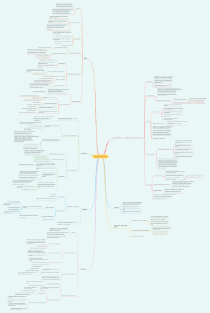
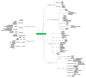
This Edraw template offers a comprehensive mind map for personnel analysis in statistical research. It starts with an overview of the basic data collection methods, including surveys, interviews, and observations. The map then branches out into key statistical concepts such as descriptive statistics, inferential statistics, and data visualization. Descriptive statistics cover measures of central tendency and dispersion, while inferential statistics delve into hypothesis testing and prediction. The template also includes sections on data interpretation and analysis, highlighting techniques for drawing meaningful insights from the collected data. Ideal for researchers, analysts, and decision-makers in human resources or related fields, this template provides a structured framework for conducting personnel analysis using statistical methods.
Edited at 2024-01-05 14:24:01
- Recommended to you
- Outline











need a detailed learning map for the stastics for people analytics including basic and advanced stastics
Basic statistics
Introduction to statistics
Definition of statistics
1. Statistics is the study of data collection, analysis, interpretation, and presentation to make meaningful conclusions in different fields, including people analytics.
2. A detailed learning map for statistics in people analytics covers both basic and advanced concepts, providing a comprehensive understanding of statistical methods and techniques.
3. Basic statistics is a fundamental component of people analytics, introducing key concepts like measures of central tendency, variability, correlation, and probability.
4. Introduction to statistics offers a foundational understanding of statistical concepts, including data types, sampling techniques, hypothesis testing, and inferential statistics.
5. Building on basic statistics, an advanced statistics course for people analytics delves into complex topics like regression analysis, multivariate analysis, predictive modeling, and data visualization.
6. Understanding advanced statistics empowers professionals in people analytics to analyze complex data sets, discover patterns, identify relationships, and make data-driven decisions.
7. By mastering both basic and advanced statistics, individuals in people analytics can effectively analyze and interpret data to gain insights, solve problems, and optimize HR strategies.
Importance of statistics in people analytics
1. Statistics is crucial in people analytics as it helps uncover patterns and trends, enabling organizations to make data-driven decisions about their workforce.
2. A comprehensive learning map for statistics in people analytics is essential, covering both basic and advanced concepts to support a deeper understanding of the subject.
3. Basic statistics should be an integral part of any learning map, providing a foundation for interpreting data and conducting basic analyses in the context of people analytics.
4. Introduction to statistics is a fundamental topic in any learning map, serving as a starting point for beginners to grasp key concepts and terminology related to people analytics.
5. By incorporating basic and advanced statistics into a learning map for people analytics, individuals can acquire the necessary skills to effectively analyze and interpret data, adding value to their organization's workforce decisions.
Overview of statistical methods
Overview of statistical methods: Provides a comprehensive understanding of statistical techniques used in people analytics, covering basic and advanced statistics.
Need a detailed learning map for statistics in people analytics: Includes both basic and advanced statistical concepts relevant to people analytics.
Basic statistics: Covers fundamental statistical concepts required for analysis in people analytics.
Introduction to statistics: Provides a basic introduction to key statistical principles used in the field of people analytics.
Descriptive statistics
Measures of central tendency (mean, median, mode)
Mean:
Average value of a set of numbers
Sum all the values and divide by the number of values
Add up all the values in the set
Count the number of values in the set
Useful for analyzing continuous and interval-level data
Median
Middle value of a sorted set of numbers
Arrange the values in numerical order
Find the middle value
If odd number of values, middle value is the median
If even number of values, average the two middle values
Resistant measure of central tendency
Not affected by extreme outliers
Suitable for skewed data or ordinal-level data
Mode
Most frequently occurring value in a dataset
Identify the value that appears the most
Count the frequency of each value
Determine the value with the highest frequency
Useful for categorical or nominal data
Can be used with other types of data, but less informative
Note: The above information provides details on the measures of central tendency - mean, median, and mode. Each measure is explained individually, breaking down the steps involved in calculating or determining the measure. Relevant information regarding the types of data suitable for each measure is also provided.
Measures of variability (range, variance, standard deviation)
Measurement of variability in data sets
Range
Definition and calculation of range
Example illustrating how to calculate range
Variance
Definition and calculation of variance
Formula for calculating variance
Example demonstrating how to compute variance
Standard deviation
Definition and calculation of standard deviation
Formula for calculating standard deviation
Example illustrating how to calculate standard deviation
Significance and interpretation of measures of variability
Importance of measures of variability in statistical analysis
Understanding the role of variability in data
Interpreting range, variance, and standard deviation values
Application of measures of variability in people analytics
Using measures of variability in analyzing HR data
Identifying patterns and trends through variability analysis
Assessing the spread of data in people analytics
Limitations and considerations
Potential limitations of measures of variability
Factors to consider when interpreting measures of variability
Comparing variability measures across different data sets
Importance of understanding measures of variability
Enhancing data analysis skills
Making informed decisions based on variability information
Improving the accuracy of statistical analyses
Resources for learning about measures of variability
Books, courses, and online tutorials on statistics
Websites and forums dedicated to statistical concepts
Practice exercises and real-world examples for applying measures of variability in analytics
1. Range, variance, and standard deviation are common measures of variability used in statistics.
2. A detailed learning map for statistics in people analytics should cover both basic and advanced concepts.
3. Basic statistics, such as mean, median, and mode, form the foundation of understanding data in people analytics.
4. Descriptive statistics provide insight into the distribution and spread of data, including measures of central tendency and variability.
5. Advanced statistics in people analytics may include regression analysis, hypothesis testing, and multivariate analysis.
6. Understanding measures of variability is crucial in analyzing and interpreting data accurately for making data-driven decisions in people analytics.
7. A comprehensive learning map should include practice exercises and real-world case studies to reinforce the understanding and application of statistical concepts in people analytics.
Frequency distributions
Definition: Frequency distributions refer to the tabular or graphical representation of data that shows the number of observations within different intervals or categories.
Tabular representation: Frequency distributions can be displayed in tables, where the intervals or categories are listed along with their corresponding frequencies.
Intervals or categories: Data is grouped into intervals or categories based on its values.
Grouping criteria: The criteria for grouping data can be determined by the researcher or based on the nature of the data.
Equal width intervals: In some cases, data may be grouped into intervals of equal width, making it easier to analyze and interpret.
Equal frequency intervals: Alternatively, data can be grouped into intervals of equal frequency, ensuring that each interval contains a similar number of observations.
Frequency column: The frequency column in a frequency distribution table represents the number of observations falling within each category or interval.
Counting method: The frequencies can be obtained by counting the occurrences of values falling in each category or interval.
Graphical representation: Frequency distributions can also be presented using graphical methods, such as histograms or bar charts.
Histogram: A histogram is a graphical representation of a frequency distribution that displays the frequencies as bars along the x-axis, with the intervals or categories represented on the y-axis.
Bar height: The height of each bar in a histogram represents the frequency or count of observations falling within the corresponding interval or category.
Bar chart: A bar chart is a similar graphical representation to a histogram, but the categories or intervals are plotted on the x-axis rather than the y-axis.
Importance of frequency distributions
Data summarization: Frequency distributions provide a concise summary of the data, allowing researchers to get a quick overview of the distribution of values.
Pattern identification: By examining the frequencies within each interval or category, patterns or trends in the data can be identified.
Data exploration: Frequency distributions help researchers explore the data and gain insights into its characteristics, such as central tendency and variability.
Comparison: Frequency distributions can be used to compare different data sets or subgroups within a larger data set.
Applications
Statistical analysis: Frequency distributions serve as a fundamental tool in various statistical analyses, such as hypothesis testing and regression analysis.
Data visualization: Graphical representations of frequency distributions help in visualizing the data and communicating the findings effectively.
Decision-making: Frequency distributions provide valuable information for making informed decisions in fields like business, healthcare, and social sciences.
Example: Suppose we have collected data on the heights of students in a class and want to create a frequency distribution.
Grouping: We can group the heights into intervals, such as 150-160 cm, 160-170 cm, etc.
Counting: Count the number of students falling within each interval to obtain the frequencies.
Tabular representation: Present the frequency distribution in a table, with intervals and corresponding frequencies.
Graphical representation: Create a histogram or bar chart to visualize the frequency distribution.
1. Understanding frequency distributions is crucial in people analytics, as it helps to analyze and interpret data accurately.
2. A detailed learning map for statistics in people analytics should cover both basic and advanced concepts to ensure a comprehensive understanding.
3. Basic statistics provides the foundation for analyzing data in people analytics, including measures of central tendency and variability.
4. Descriptive statistics enables us to summarize and describe data from a people analytics perspective, such as through graphical representations and numerical summaries.
5. To excel in people analytics, a thorough understanding of basic and advanced statistics is essential, as it allows for more sophisticated analysis and insights.
6. Exploring concepts like correlation, regression, hypothesis testing, and statistical modeling are part of the advanced statistics required for people analytics.
7. By combining basic and advanced statistics, a comprehensive learning map will equip individuals with the necessary skills to effectively analyze data and draw meaningful conclusions in the field of people analytics.
Graphical representation of data (histograms, bar charts, pie charts)
Inferential statistics
Sampling techniques
Creating a detailed learning map for statistics in people analytics, encompassing both basic and advanced statistics, is essential for mastering this field. As the demand for people analytics continues to grow, it is crucial to have a solid understanding of statistical concepts and techniques to make informed decisions and provide valuable insights. Firstly, one should start with the basics of statistics, such as descriptive statistics, probability, and inferential statistics. Descriptive statistics enables understanding and summarizing data through measures like mean, median, and standard deviation. Probability provides a foundation for understanding random events
Random sampling
Involves selecting a sample in which every member of the population has an equal chance of being chosen.
This reduces bias and ensures representative results.
Stratified sampling
Divides the population into relevant groups or strata and then selects samples from each stratum.
Ensures representation from different groups within the population.
Cluster sampling
Involves dividing the population into clusters or naturally occurring groups.
Selects specific clusters for sampling instead of individual members.
Helpful when the population is too large or geographically dispersed.
systematic sampling
Selects samples at regular intervals from a population list.
Requires a predetermined sample interval and starting point.
Convenience sampling
Involves selecting samples based on convenience or easy accessibility.
Often used when time or resources are limited.
Snowball sampling
Starts with an initial sample and expands by asking participants to refer others.
Useful for studying hard-to-reach populations or sensitive topics.
Quota sampling
Ensures specific quotas or proportions of individuals from different subgroups are included in the sample.
Allows for representation of different subgroups, but may introduce bias if quotas are not accurately defined.
(Note: The above content does not provide a summary.)
Hypothesis testing
Definition and purpose of hypothesis testing
Hypothesis testing is a statistical procedure used to make inferences about a population based on sample data.
The purpose of hypothesis testing is to determine if there is enough evidence to support or reject a claim or hypothesis about a population parameter.
Steps in hypothesis testing
Step 1: State the null and alternative hypotheses
The null hypothesis (H0) represents the assumption of no difference or no effect.
The alternative hypothesis (Ha) represents the claim or hypothesis that we are trying to find evidence for.
Step 2: Set the significance level (alpha)
The significance level, commonly denoted as alpha (α), determines the probability of rejecting the null hypothesis when it is true. It controls the trade-off between Type I and Type II errors.
Step 3: Calculate the test statistic
The test statistic is a measure of how far the sample estimate is from the hypothesized value, assuming the null hypothesis is true.
Step 4: Determine the critical region and calculate the p-value
The critical region is the range of values that, if the test statistic falls within, leads to rejection of the null hypothesis.
The p-value is the probability of obtaining a test statistic as extreme as, or more extreme than, the observed data, assuming the null hypothesis is true.
Step 5: Make a decision and draw conclusions
If the test statistic falls within the critical region, reject the null hypothesis, and conclude that there is sufficient evidence to support the alternative hypothesis.
If the test statistic does not fall within the critical region, fail to reject the null hypothesis, and conclude that there is not enough evidence to support the alternative hypothesis.
Types of hypothesis tests
One-sample t-test
Used to compare the mean of a single sample to a known or hypothesized population mean.
Independent samples t-test
Used to compare the means of two independent samples to determine if they are significantly different from each other.
Paired samples t-test
Used to compare the means of two related samples, such as before and after measurements on the same subjects.
Chi-square test
Used to determine if there is a significant association between two categorical variables.
ANOVA (Analysis of Variance)
Used to compare the means of three or more groups to determine if there are significant differences among them.
Key concepts in hypothesis testing
Type I error
Occurs when the null hypothesis is rejected when it is actually true, leading to a false positive conclusion.
Type II error
Occurs when the null hypothesis is not rejected when it is actually false, leading to a false negative conclusion.
Power
The probability of correctly rejecting the null hypothesis when it is false. Higher power means a higher chance of detecting a true effect.
Sample size and statistical power
Larger sample sizes generally lead to higher statistical power, increasing the likelihood of detecting a true effect.
Confidence intervals
A range of values within which the true population parameter is estimated to fall, with a certain level of confidence. Confidence intervals can be used in conjunction with hypothesis testing.
Confidence intervals
Definition and concept of confidence intervals
Confidence interval is a range of values that is used to estimate an unknown population parameter based on a sample statistic.
It provides a measure of uncertainty or variability in the estimated parameter.
Calculation of confidence intervals
Confidence intervals are calculated using a specific level of confidence and the standard error of the sample statistic.
The level of confidence determines the likelihood that the interval contains the true population parameter.
The standard error is a measure of the variability or uncertainty in the sample statistic.
Commonly used formulas for confidence intervals include those for means, proportions, and differences between means or proportions.
Interpreting confidence intervals
Confidence intervals provide a range of plausible values for the population parameter.
The wider the interval, the less precise the estimate.
If the interval includes the hypothesized value, we fail to reject the null hypothesis.
If the interval does not include the hypothesized value, we reject the null hypothesis.
Confidence intervals can also be used to compare two different groups or conditions.
Factors affecting the width of confidence intervals
Sample size: Larger sample sizes generally result in narrower confidence intervals as they reduce the variability in the sample statistic.
Level of confidence: Higher confidence levels necessitate wider intervals to capture a greater range of values.
Standard deviation: A larger standard deviation leads to wider confidence intervals as it indicates greater variability in the data.
Applications of confidence intervals
Confidence intervals are widely used in statistical analysis to estimate population parameters and make inferences about the population.
They are commonly used in hypothesis testing, comparing means or proportions, and predicting future values.
In people analytics, confidence intervals can be used to estimate employee satisfaction levels, identify significant differences in performance metrics, or assess the effectiveness of training programs.
Regression analysis
Definition and introduction
Regression analysis is a statistical technique used to model the relationship between a dependent variable and one or more independent variables.
The goal is to understand how changes in the independent variables affect the dependent variable.
Types of regression analysis
Simple linear regression
Involves one dependent variable and one independent variable
Assumes a linear relationship between the variables
Used to predict the value of the dependent variable based on the independent variable
Multiple regression
Involves one dependent variable and two or more independent variables
Allows for the analysis of multiple factors that may affect the dependent variable
Helps to identify the individual contributions of each independent variable to the dependent variable
Logistic regression
Used when the dependent variable is categorical or binary
Predicts the probability of an event occurring
Useful in classification problems
Assumptions of regression analysis
Linearity: Assumes a linear relationship between the variables
Independence: Assumes the observations are independent of each other
Homoscedasticity: Assumes equal variance of errors
Normality: Assumes the errors are normally distributed
Steps in regression analysis
Data collection and preprocessing
Gather data on the dependent and independent variables
Clean and transform the data
Handle missing values and outliers
Model specification
Determine the type of regression analysis to be used
Select the independent variables to include in the model
Specify the functional form of the relationship (linear, quadratic, etc.)
Estimation and evaluation
Estimate the model parameters using statistical methods
Assess the goodness of fit of the model
Evaluate the significance of the independent variables
Interpretation and prediction
Interpret the estimated coefficients and their significance
Use the model to make predictions or inferences
Applications of regression analysis
Economic forecasting
Predicting GDP growth based on factors such as interest rates and inflation
Marketing research
Predicting sales based on advertising expenditure and customer demographics
Health outcomes research
Predicting patient outcomes based on treatment variables and patient characteristics
Financial analysis
Predicting stock prices based on market variables and company fundamentals
Limitations of regression analysis
Linearity assumption may not hold in real-world scenarios
Reliance on correlation rather than causation
Sensitivity to outliers and influential observations
Overfitting if too many variables are included without proper justification
Practical applications of basic statistics in people analytics
Analyzing employee satisfaction surveys
Collecting survey data
Determining survey questions
Designing questions to measure employee satisfaction
Ensuring questions are clear and unambiguous
Selecting survey methods
Choosing between online surveys, paper-based surveys, or in-person interviews
Considering factors such as privacy and anonymity
Determining the sample size
Calculating the number of participants needed for statistical significance
Balancing the need for accuracy with practical constraints
Data cleaning and preparation
Removing incomplete or inconsistent responses
Checking for data entry errors and missing values
Standardizing response scales for ease of analysis
Transforming qualitative responses into quantitative data
Exploratory data analysis
Descriptive statistics
Calculating measures of central tendency (mean, median, mode)
Examining variability (range, standard deviation)
Understanding the distribution of responses (histograms, boxplots)
Data visualization
Creating charts and graphs to visually represent survey data
Identifying patterns and trends in employee satisfaction levels
Identifying outliers and unusual patterns in the data
Inferential statistics
Hypothesis testing
Formulating null and alternative hypotheses
Selecting an appropriate test statistic (t-test, chi-square test)
Interpreting p-values and making conclusions
Correlation analysis
Examining relationships between satisfaction and other variables
Calculating correlation coefficients (Pearson's r, Spearman's rho)
Assessing the strength and direction of correlations
Applying results to people analytics
Drawing insights and implications from the data analysis
Identifying areas for improvement in employee satisfaction
Making data-driven decisions to enhance employee engagement
Monitoring and evaluating the effectiveness of interventions
Understanding workforce demographics
Definition and importance of workforce demographics
Workforce demographics refer to the characteristics and composition of a company's employees.
Understanding workforce demographics is crucial for effective people analytics.
Basic statistics for analyzing workforce demographics
Descriptive statistics
Measures of central tendency (mean, median, mode) reveal the average or typical values of demographic variables.
Measures of dispersion (variance, standard deviation) indicate the spread or variability in demographic data.
Graphical representation
Bar charts, pie charts, and histograms can visually display workforce demographics.
Scatter plots and line graphs illustrate relationships between demographic variables.
Advanced statistics for analyzing workforce demographics
Inferential statistics
Hypothesis testing helps determine if there are significant differences or relationships in demographic data.
Regression analysis examines the impact of one or more variables on a demographic outcome.
Multivariate analysis
Factor analysis identifies underlying factors that explain patterns in demographic variables.
Cluster analysis categorizes employees into distinct groups based on demographic characteristics.
Practical applications of basic statistics in people analytics
Benchmarking workforce demographics
Comparing demographic data against industry or regional norms helps identify areas for improvement.
Monitoring changes in workforce demographics over time aids in measuring diversity and inclusion efforts.
Identifying talent gaps and recruitment strategies
Analyzing demographic profiles of high-performing employees assists in identifying desired traits for recruitment.
Identifying gaps in representation and designing targeted recruitment strategies to enhance diversity.
Evaluating the effectiveness of diversity and inclusion initiatives
Statistical analysis can measure the impact of diversity programs on hiring, promotion, and retention.
Examining demographic distributions within different levels of the organization helps assess inclusive practices.
Predicting employee turnover and engagement
Correlating demographic variables with turnover rates or engagement surveys can identify risk factors.
Applying predictive modeling techniques to forecast future turnover or engagement levels based on demographic data.
Introduction to predictive modeling techniques in people analytics
Explanation of predictive modeling techniques
Various predictive modeling techniques used in people analytics (e.g. regression analysis, decision trees, machine learning)
Definition and overview of regression analysis
Explanation of decision trees and their applications in people analytics
Introduction to machine learning and its relevance in predicting turnover or engagement levels
Examples of predictive modeling techniques used in workforce analytics
Importance of utilizing demographic data in predictive modeling
Overview of demographic data in people analytics
Definition and types of demographic data (e.g. age, gender, education level)
Explanation of the relevance of demographic data in predicting turnover or engagement levels
Importance of collecting and analyzing accurate demographic data
Methods of incorporating demographic data into predictive models
Techniques for data preprocessing and cleaning
Strategies for feature engineering and selection
Integration of demographic variables into predictive models
Practical applications of predictive modeling in people analytics
Case studies and examples of using predictive modeling to forecast turnover or engagement levels
Examination of real-life scenarios and their predictive modeling solutions
How predictive modeling can assist in identifying high-risk employees for turnover
Application of predictive modeling in understanding engagement drivers and predicting future engagement levels
Predictive modeling's role in identifying potential attrition patterns based on demographic factors
Benefits and limitations of using predictive modeling in people analytics
Advantages of accurate turnover or engagement predictions for effective decision-making
Challenges and considerations in implementing and interpreting predictive modeling results
Steps to build and deploy predictive models in people analytics
Overview of the predictive modeling process
Data collection and preparation for modeling
Selection of appropriate modeling techniques
Training and evaluation of predictive models
Deployment and integration of models into people analytics systems
Recommendations for successful implementation of predictive modeling in an organization
Collaboration between HR and data analytics teams
Continuous monitoring and updating of predictive models
Ethical considerations and privacy protection in utilizing demographic data for predictive modeling
Evaluating performance metrics
Definition and importance of performance metrics
Performance metrics are quantitative measures used to evaluate the performance of individuals, teams, or organizations in achieving their goals.
They play a crucial role in assessing and improving performance in various fields.
Types of performance metrics
Outcome-based metrics focus on the final results or output achieved.
Examples include sales revenue, customer satisfaction scores, and employee turnover rates.
Process-based metrics measure the efficiency and effectiveness of the processes involved.
Examples include cycle time, productivity ratios, and error rates.
Input-based metrics assess the resources allocated or invested in achieving the desired outcomes.
Examples include budget utilization, employee training hours, and equipment utilization.
Key considerations in evaluating performance metrics
Reliability and validity
Metrics should be consistently measured and accurately reflect the intended aspects of performance.
Adequate measurement tools and methods should be used to ensure data quality.
Alignment with goals and objectives
Performance metrics should be aligned with the specific goals and objectives of the people analytics process.
They should provide meaningful insights and indicators of progress towards desired outcomes.
Relevance and specificity
Metrics should be relevant to the specific context and purpose of the evaluation.
They should provide specific and actionable information for decision-making and improvement.
Comparative analysis
Metrics should allow for benchmarking and comparison against standards, targets, or industry best practices.
Comparative analysis helps identify areas for improvement and facilitates performance reviews.
Challenges and limitations in evaluating performance metrics
Subjectivity and bias
Evaluators may have different interpretations or biases when assessing performance metrics.
Measures should be standardized and calibrated to minimize subjectivity.
Data quality and availability
Availability and accuracy of data can impact the reliability and effectiveness of performance metrics.
Adequate data collection processes and systems should be in place to ensure data availability and quality.
Interdependencies and confounding factors
Performance metrics may be influenced by various external factors or internal factors that are not directly controllable.
Analytical techniques should be employed to identify and account for confounding factors.
Lagging indicators
Some performance metrics may be lagging indicators, reflecting past performance rather than current or future performance.
Leading indicators should also be considered to provide more forward-looking insights.
(Note: This is a detailed breakdown of the topics and subtopics within the outline "Evaluating performance metrics" for the statistics for people analytics learning map, as requested. It provides a comprehensive overview of the key aspects related to evaluating performance metrics, including their definition, types, considerations, challenges, and limitations.)
Advanced statistics
Multivariate analysis
Introduction to multivariate analysis techniques
Definition and importance of multivariate analysis techniques
Multivariate analysis techniques refer to statistical methods used to analyze data sets with multiple variables.
It is important in various fields like finance, marketing, healthcare, and social sciences as it allows for a comprehensive analysis of relationships between multiple variables.
Basic concepts in multivariate analysis
Understanding of variables
Different types of variables, including categorical and continuous variables.
Roles of dependent and independent variables in multivariate analysis.
Data collection and preparation
Gathering data from multiple sources.
Handling missing data and outliers.
Scaling and standardizing variables for analysis.
Exploratory data analysis techniques
Summary statistics
Calculation and interpretation of mean, median, mode, and standard deviation.
Understanding skewness and kurtosis.
Data visualization
Creating histograms, scatter plots, and box plots.
Interpreting patterns and relationships between variables.
Correlation analysis
Calculating correlation coefficients (e.g., Pearson, Spearman).
Assessing the strength and direction of relationships between variables.
Multivariate regression analysis
Introduction to regression analysis
Understanding the concept of regression.
Types of regression models (e.g., linear, logistic).
Building and interpreting regression models
Selecting independent variables.
Interpreting coefficients and their significance.
Assessing model fit and goodness of fit.
Handling multicollinearity
Identifying and dealing with correlated independent variables.
Multivariate analysis of variance (MANOVA)
Introduction to MANOVA
Understanding the concept and purpose of MANOVA.
Differences between ANOVA and MANOVA.
Conducting MANOVA
Selecting dependent and independent variables.
Interpreting the results, including group differences and interactions.
Post-hoc analysis
Performing follow-up tests (e.g., Tukey's HSD, Bonferroni) to identify specific group differences.
Principal component analysis (PCA)
Overview of PCA
Understanding the concept and purpose of PCA.
Identifying variables with the most variance.
Conducting PCA
Standardizing variables for analysis.
Interpreting factor loadings and eigenvalues.
Determining the number of principal components to retain.
Factor analysis
Introduction to factor analysis
Understanding the concept and purpose of factor analysis.
Differences between exploratory and confirmatory factor analysis.
Conducting factor analysis
Selecting variables and factors.
Interpreting factor loadings and communalities.
Assessing reliability and validity of factors.
Cluster analysis
Overview of cluster analysis
Understanding the concept and purpose of cluster analysis.
Different types of clustering algorithms (e.g., hierarchical, k-means).
Conducting cluster analysis
Selecting variables and distance measures.
Interpreting dendrograms and cluster assignments.
Assessing the quality of clustering solutions.
Discriminant analysis
Introduction to discriminant analysis
Understanding the concept and purpose of discriminant analysis.
Differences between discriminant analysis and logistic regression.
Performing discriminant analysis
Selecting dependent and independent variables.
Interpreting discriminant functions and group separations.
Assessing classification accuracy and overall model performance.
Factor analysis
Definition and purpose
Factor analysis is a statistical technique that aims to identify underlying factors or dimensions in a larger set of observed variables.
It is used to reduce the dimensionality of data and explore the relationships between variables.
Basic concepts
Variables: The observed variables that are used in the factor analysis.
Factors: The underlying dimensions or latent variables that explain the patterns observed in the variables.
Steps involved in factor analysis
Determine the objectives: Define the research goals and identify the variables to be included in the analysis.
Data collection: Gather the data for the selected variables.
Data screening: Check the data for missing values, outliers, and normality assumptions.
Factor extraction: Identify the factors that explain the most variance in the data.
Factor rotation: Rotate the factors to simplify the interpretation and improve clarity.
Factor interpretation: Assign meaningful labels to the factors based on the pattern of loadings.
Types of factor analysis
Exploratory factor analysis (EFA): Used when the researcher wants to explore the underlying structure of the variables.
Confirmatory factor analysis (CFA): Used when the researcher has specific hypotheses about the factor structure and wants to test them using the collected data.
Applications of factor analysis
Dimension reduction: Factor analysis can help researchers reduce the number of variables by identifying the underlying dimensions in the data.
Scale development: It is often used to develop psychometric scales by identifying and validating the underlying factors.
Market research: Factor analysis can be used to analyze consumer preferences and identify the key factors influencing brand perception.
Psychological research: It is commonly used in psychology to study personality traits and psychological constructs.
Software tools for factor analysis
There are several software packages available to perform factor analysis, such as SPSS, SAS, R, and Stata.
These tools provide a range of options and techniques for factor extraction, rotation, and interpretation.
Common challenges in factor analysis
Determining the number of factors: It can be difficult to determine the optimal number of factors to extract from the data.
Interpreting factor loadings: Interpreting the meaning of the factors and their relationships with the observed variables can be subjective.
Assessing model fit: Evaluating the adequacy of the factor model requires considering fit indices and comparing alternative models.
Resources for learning factor analysis
Books: "Exploratory Factor Analysis" by Leech et al., "Factor Analysis and Related Methods" by Abdi and Williams.
Online courses: Platforms like Coursera and Udemy offer courses on factor analysis and multivariate analysis.
Research papers: Reading published studies that have used factor analysis can provide practical insights into its applications.
Cluster analysis
Definition and purpose
Cluster analysis is a statistical technique used to identify groups or clusters within a dataset based on similarity or proximity.
It helps in understanding patterns, relationships, and structures within the data.
It can be used for various purposes such as segmentation, classification, and anomaly detection.
Types of cluster analysis
Hierarchical clustering
In hierarchical clustering, data objects are grouped into a hierarchy of clusters based on their similarity.
Two main approaches are agglomerative clustering and divisive clustering.
Agglomerative clustering starts with each data point as a separate cluster and merges them iteratively based on similarity.
Divisive clustering starts with all data points in a single cluster and splits them into smaller clusters based on dissimilarity.
Partitioning clustering
In partitioning clustering, data objects are divided into non-overlapping clusters where each object belongs to only one cluster.
Popular methods include k-means, k-medoids, and Gaussian mixture models.
The choice of the number of clusters (k) is important and various techniques such as elbow method and silhouette analysis can be used.
Density-based clustering
Density-based clustering groups data objects based on the density of data points in the feature space.
It can automatically discover clusters of arbitrary shape and handle noise in the data.
DBSCAN (Density-Based Spatial Clustering of Applications with Noise) is a well-known density-based clustering algorithm.
Key steps in cluster analysis
Data preprocessing
Convert categorical variables to numerical representation if necessary.
Handle missing data by imputation or deletion.
Standardize or normalize the variables if needed.
Selecting similarity/distance measure
Choose an appropriate measure to quantify the similarity or dissimilarity between data objects.
Examples include Euclidean distance, Manhattan distance, and cosine similarity.
Choosing the number of clusters
Determine the optimal number of clusters based on domain knowledge or using evaluation metrics.
Elbow method, silhouette analysis, and hierarchical clustering dendrogram can help in this process.
Selecting clustering algorithm
Choose a suitable clustering algorithm based on the type of data, desired cluster structure, and computational efficiency.
Consider the assumptions and limitations of each algorithm.
Interpreting and evaluating clusters
Analyze and interpret the obtained clusters based on the characteristics and attributes of the data.
Evaluate the quality of clusters using internal and external validation measures.
Internal measures assess the compactness and separation of clusters.
External measures compare the cluster assignments with known class labels or ground truth.
Applications of cluster analysis in people analytics
Employee segmentation
Cluster analysis can be used to segment employees based on characteristics such as performance, demographics, or engagement level.
This segmentation can provide insights for targeted HR interventions and personalized talent management strategies.
Employee turnover prediction
By clustering employees based on relevant features and past turnover patterns, it is possible to identify groups at higher risk of leaving the organization.
This information can guide retention efforts and help in developing proactive retention strategies.
Talent development and succession planning
Clustering employees based on their skills, competencies, or performance can aid in talent identification and succession planning.
It facilitates the identification of high-potential employees and assists in designing development programs tailored to specific groups.
Workforce diversity analysis
Cluster analysis can be applied to analyze diversity within the workforce by grouping employees based on characteristics such as gender, ethnicity, or education.
It helps in identifying areas where diversity and inclusion initiatives may be needed and evaluating their effectiveness.
Employee sentiment analysis
By clustering employees based on sentiment expressed in feedback surveys or social media posts, it is possible to understand common themes and sentiments among different groups.
This analysis can inform HR strategies related to employee satisfaction, engagement, and well-being.
Discriminant analysis
Definition: Discriminant analysis is a statistical technique used to identify the underlying factors that differentiate between two or more groups or populations.
It helps to understand the relationships between variables and groups.
By examining the differences between groups, it provides insights into the factors that contribute to those differences.
These factors can be used to classify future observations or individuals into specific groups.
Discriminant analysis is widely used in various fields, including people analytics, to analyze and predict group membership.
It is particularly useful in HR and people analytics to understand the factors that influence employee performance, engagement, or attrition.
By analyzing different variables related to employees, such as demographics, skills, and performance metrics, discriminant analysis can identify the key factors that distinguish high-performing employees from low-performing ones.
This information can then be used to make data-driven decisions and strategies for talent management and organizational development.
Assumptions and requirements
Groups should be clearly defined and mutually exclusive.
The independent variables should be continuous or discrete variables that can be measured numerically.
The variables should be normally distributed within each group.
The variance-covariance matrices of the groups should be equal.
Steps involved in conducting discriminant analysis
1. Data preparation
Collect relevant data for the analysis, including variables related to the groups of interest.
Ensure the data is properly cleaned and formatted.
2. Test assumptions
Check if the assumptions for discriminant analysis are met.
If not, appropriate transformations or alternative methods may be needed.
3. Variable selection
Determine which variables to include in the analysis based on their potential discriminatory power.
Use statistical techniques like correlation analysis or stepwise regression to identify the most important variables.
4. Model estimation
Use statistical software to estimate the discriminant function(s).
The discriminant function(s) will provide coefficients and weights for each variable.
5. Model validation and interpretation
Evaluate the discriminant function(s) for their predictive power and accuracy.
Interpret the discriminant function(s) to understand the relative importance of variables and how they contribute to group differentiation.
6. Classification of new observations
Apply the discriminant function(s) to classify new observations or individuals into appropriate groups.
Applications of discriminant analysis in people analytics
Employee performance analysis
By employing discriminant analysis, HR professionals can identify the key factors that differentiate high-performing employees from others.
This insight can be used to develop targeted training programs or interventions to improve overall employee performance.
Attrition prediction
Discriminant analysis helps organizations understand the factors that contribute to employee attrition.
By identifying the warning signs of attrition, organizations can take preventive measures and implement retention strategies.
Employee engagement analysis
By analyzing various variables, such as job satisfaction, work-life balance, and career development opportunities, discriminant analysis can identify the factors that impact employee engagement.
This understanding can guide the design of initiatives to enhance employee engagement and satisfaction.
Talent segmentation and recruitment
Discriminant analysis can help in classifying applicants or candidates into different talent segments.
By identifying the attributes that distinguish high-potential candidates, organizations can make informed decisions during the recruitment process to select the best-fit candidates.
Limitations and considerations
Discriminant analysis assumes linear relationships between variables and group membership.
Violation of assumptions, such as non-normality or unequal variance-covariance matrices, can impact the validity of results.
It is essential to select appropriate variables and conduct rigorous data analysis to ensure meaningful and accurate results.
Discriminant analysis should be used in conjunction with other statistical techniques and qualitative insights to gain a comprehensive understanding of the factors influencing group differentiation.
Time series analysis
Forecasting techniques
Introduction to forecasting techniques
Definition and importance of forecasting
Role of forecasting in people analytics
Benefits of accurate forecasting
Basic forecasting techniques
Moving averages method
Definition and concept of moving averages
Moving averages is a statistical technique used to analyze and smooth out fluctuations or noise in time series data.
It is a common method used in forecasting and trend analysis.
Moving averages calculate the average value of a subset of data points within a given time period to create a single value.
The time period can be days, weeks, months, or any other interval depending on the data being analyzed.
The subset of data points is typically selected based on a sliding window approach.
Moving averages can be classified into different types
Simple moving average (SMA)
SMA is the most basic form of moving averages that calculates the average of a fixed number of data points.
For example, a 7-day SMA calculates the average of the last seven data points.
This method assigns equal weight to each data point in the subset.
Weighted moving average (WMA)
WMA assigns different weights to each data point in the subset based on their importance or relevance.
This means that some data points have a greater impact on the moving average value than others.
The weights can be assigned in a linear or exponential manner.
Exponential moving average (EMA)
EMA is a type of moving average that puts more weight on recent data points.
It uses an exponentially decreasing weight for each data point, giving more significance to recent observations.
As a result, EMA is more responsive to short-term changes in the data compared to SMA or WMA.
Cumulative moving average (CMA)
CMA calculates the average of all data points up to a specific point in time.
It is commonly used to monitor the historical progress of a variable over time.
Moving averages have several applications in statistics and analytics
Trend analysis
Moving averages can help identify and analyze trends in time series data.
By smoothing out the noise, they reveal the underlying patterns and direction of the data.
Forecasting
Moving averages are often used in forecasting future values based on historical data.
They provide a simple yet effective method for predicting trends and making short-term projections.
Seasonal adjustment
Moving averages can aid in identifying and removing seasonal variations from time series data.
This allows for a clearer understanding of the underlying long-term trend.
Data smoothing
Moving averages can be used to reduce random fluctuations or irregularities in data.
They help create a more stable and consistent representation of the data.
This is particularly useful when dealing with noisy or erratic data.
Calculation process of simple moving averages
What is a simple moving average?
Definition: A simple moving average (SMA) is a statistical calculation used to analyze data points over a specific period of time.
How is it calculated?
Step 1: Determine the time period for the moving average (e.g., 10 days).
Step 2: Add up the data points for the specified time period.
Step 3: Divide the sum by the number of data points in the time period to obtain the average.
Importance of simple moving averages
Helps identify trends and patterns in data.
Smoothens out fluctuations to reveal underlying patterns.
Used in various fields for forecasting, trend analysis, and decision-making.
Steps to calculate simple moving averages
Step 1: Compile the data points for the specified time period (e.g., daily closing prices of a stock for 10 days).
Step 2: Add up the data points.
Step 3: Divide the sum by the number of data points to obtain the average.
Step 4: Repeat steps 1-3 for subsequent time periods.
Example application of simple moving averages in financial analysis
Calculate 10-day simple moving averages of a stock.
Gather the closing prices for the stock for the past 10 days.
Add up the closing prices.
Divide the sum by 10 to determine the 10-day moving average.
Repeat the process for subsequent days to track the moving average over time.
Limitations of simple moving averages
Ignores older data points as new ones are added, leading to lagging indicators.
Can be sensitive to outliers or sudden price fluctuations.
May not work well for volatile or cyclical data.
Considered a basic forecasting technique, not suitable for complex analysis.
Advantages and limitations of moving averages method
Advantages
Helps in smoothing out fluctuations in time series data.
Moving averages method calculates an average of a specified number of consecutive data points, thus reducing random variation.
This helps to identify underlying trends or patterns in the data.
Provides a simple and easy-to-understand forecasting technique.
The method is straightforward to implement and interpret, making it accessible for beginners.
It does not require complex statistical calculations or assumptions.
Helps in identifying significant changes in the data.
By applying moving averages over different time periods, sudden changes or outliers in the data can be identified.
Useful for short-term forecasting.
Moving averages are particularly effective for forecasting data with short-term patterns or fluctuations.
It can be used to forecast sales, inventory levels, or other time-dependent variables in the near future.
Limitations
Smoothes out sharp changes or abrupt shifts in the data.
Moving averages method tends to delay the detection of sudden changes in the time series data.
It smooths out sharp spikes or dips in the data, making it difficult to capture sudden shifts accurately.
Ignores other important factors or variables.
Moving averages focus solely on historical data to make forecasts.
It does not consider other relevant factors like seasonality, trends, or external influences that may impact the data.
May not be suitable for long-term forecasting.
When forecasting over longer periods, moving averages might be less accurate due to their inability to capture long-term trends.
It may fail to account for structural changes or evolving patterns in the data.
Vulnerable to outliers or irrelevant data points.
A single outlier or irrelevant data point can significantly distort moving average forecasts.
It may result in misleading predictions if the data contains extreme values or unusual events.
Remember, this is only a detailed breakdown of the advantages and limitations of the moving averages method for people analytics statistics.
Exponential smoothing method
Understanding exponential smoothing technique
Definition and basics of exponential smoothing technique
Exponential smoothing is a time series forecasting method used to predict future values based on past observations.
It assigns exponentially decreasing weights to past observations, with the most recent observation having the highest weight.
The technique is popular due to its simplicity and effectiveness in capturing trends and seasonal patterns.
Types of exponential smoothing methods
Simple exponential smoothing
Simple exponential smoothing is a basic form of exponential smoothing that considers only the current observation and the previous forecast.
It is suitable for time series data without any trend or seasonal patterns.
Holt's linear exponential smoothing
Holt's linear exponential smoothing extends simple exponential smoothing by incorporating a trend component.
It uses two smoothing parameters, one for the level (α) and one for the trend (β).
This method is useful for time series data with a linear trend.
Holt-Winters' seasonal exponential smoothing
Holt-Winters' seasonal exponential smoothing extends Holt's linear exponential smoothing by incorporating seasonality.
It includes smoothing parameters for the level (α), trend (β), and seasonal component (γ).
This method is suitable for time series data with both trend and seasonality.
Advantages and limitations of exponential smoothing technique
Advantages
Exponential smoothing is easy to understand and implement.
It provides accurate forecasts for time series data with trends and seasonal patterns.
The technique is computationally efficient, making it suitable for large-scale forecasting.
Limitations
Exponential smoothing assumes that past observations have equal importance, which may not always be the case.
It cannot handle time series data with abrupt changes or outliers effectively.
The method may require manual adjustment of smoothing parameters to obtain optimal forecasts.
Calculation formula for exponential smoothing
Definition and basic concept
Exponential smoothing is a time series forecasting method used to predict future values based on a weighted average of past observations.
Calculation steps
Step 1: Start with an initial forecast for the first period.
Step 2: Calculate the smoothing factor (alpha) which determines the weight of the most recent observation. It is typically a value between 0 and 1.
Step 3: For each subsequent period, use the following formula to calculate the forecast
Forecast for period t = α * Observation for period t + (1-α) * Forecast for period (t-1)
Step 4: Repeat step 3 for all periods in the time series.
Interpretation and significance of the formula
The formula calculates the forecast for each period by giving more weight to recent observations and less weight to older ones, thereby capturing the trend and smoothing out random fluctuations.
Factors influencing the forecast accuracy
The selection of the smoothing factor (alpha) plays a crucial role in the accuracy of the forecast. A higher alpha value gives more weight to recent observations, making the forecast more responsive to changes but potentially less stable. Conversely, a lower alpha value provides more smoothing, making the forecast more stable but potentially less sensitive to recent changes. The choice of alpha depends on the characteristics of the time series and the specific forecasting goals.
Example
Let's say we have monthly sales data and want to forecast the sales for the next month. We start with an initial forecast and a chosen smoothing factor (alpha = 0.3).
Month 1: Initial forecast = 1000
Month 2: Observed sales = 1200
Month 2 forecast = 0.3 * 1200 + 0.7 * 1000 = 1170
Month 3: Observed sales = 1250
Month 3 forecast = 0.3 * 1250 + 0.7 * 1170 = 1191
Repeat the calculation for subsequent periods.
Advantages and limitations of exponential smoothing
Advantages
Simple and easy to understand.
Flexibility to adapt to different time series patterns.
Quick calculation and responsiveness to recent changes.
Limitations
Assumes a linear trend and can struggle with irregular or non-linear patterns.
Relies heavily on the choice of the smoothing factor, which can be subjective.
Does not consider external factors or causal relationships.
Advantages and limitations of exponential smoothing method
Time series decomposition method
Definition and purpose of time series decomposition
Definition: Time series decomposition refers to the process of breaking down a time series into its individual components, namely trend, seasonality, and random fluctuation, in order to better understand and analyze its underlying patterns.
Trend: The trend component represents the long-term change or direction of a time series. It indicates whether the time series is increasing, decreasing, or remaining stable over time.
Content: Trend analysis helps in identifying overall patterns or patterns that occur over a longer period, enabling better decision-making and forecasting.
Content: Trend can be analyzed using various methods such as moving averages, linear regression, or exponential smoothing techniques.
Seasonality: The seasonal component represents the recurrent patterns or variations that occur within a specific time frame, such as daily, weekly, or yearly cycles.
Content: Analyzing seasonality allows for understanding recurring patterns and making informed decisions based on the time of the year or specific time intervals.
Content: Techniques like seasonal decomposition of time series (SATS) or Fourier analysis can be used to identify and extract the seasonal component.
Random fluctuation: Also known as the residual or error component, it represents the unpredictable or random variation in a time series after removing the trend and seasonality.
Content: Analyzing random fluctuation helps in understanding the unpredictable or irregular events or variations that might occur in a time series.
Content: Residual analysis can be performed to check for any remaining patterns or structures in the time series after decomposition.
Components of time series decomposition
Trend
The long-term movement or direction of the time series.
It represents the overall pattern or growth/decline in the data.
It helps identify the underlying trend for planning and forecasting.
Trend estimation techniques include
Moving averages: Averages of data over a specific time period to identify trend patterns.
Linear regression: Fitting a straight line to the data points to represent the trend.
Seasonality
The repetitive and predictable pattern that occurs within a fixed time period.
It captures regular variations in the data due to seasonal factors.
It helps understand the cyclical nature of the time series and its impact on forecasting.
Seasonality identification methods include
Seasonal subseries plot: Dividing the time series into smaller seasonal subseries for analysis.
Autocorrelation function (ACF) plot: Examining correlation patterns at different lags to detect seasonality.
Cyclical variations
Longer-term fluctuations in the time series that are not strictly related to seasonality.
It represents economic, business, or societal factors influencing the data.
It helps identify larger cycles or business cycles within the time series.
Cyclical variations can be identified through techniques such as
Spectral analysis: Examining the frequency components of the time series using Fourier transform.
Hodrick-Prescott (HP) filter: Decomposing the time series into cyclical and trend components.
Irregular or random variations
The unpredictable and erratic fluctuations that cannot be attributed to trend, seasonality, or cyclical factors.
It captures the residual variability or noise in the time series.
It helps assess the randomness or uncertainty in the data.
Irregular variations can be analyzed through
Residual analysis: Examining the difference between the observed and estimated values in a time series model.
Statistical tests for randomness: Checking if the residuals follow a particular pattern or distribution.
Steps involved in time series decomposition
Introduction to time series decomposition
Definition and importance of time series decomposition
Explanation of seasonal and trend components
Overview of additive and multiplicative decomposition methods
Data preparation for time series decomposition
Selection of appropriate time series data
Handling missing values and outliers
Resampling or interpolation techniques, if necessary
Identification of seasonal component
Calculation of seasonal indices
Seasonality detection using moving averages or other methods
Evaluation of the seasonality strength and pattern
Extraction of trend component
Application of smoothing techniques like moving averages or exponential smoothing
Removal of short-term fluctuations and noise from the time series
Evaluation of the trend stability and direction
Removal of irregular or random component
Computation of residuals or error terms
Evaluation of the randomness and variability of the residuals
Analysis of autocorrelation and presence of outliers in the residuals
Evaluation and validation of time series decomposition
Assessment of the decomposed components' contribution to the overall time series
Comparison of the decomposed series with the original series
Evaluation of the quality and accuracy of the decomposition technique used
Purpose of time series decomposition
Content: Decomposing a time series helps in understanding the individual components' contributions, making it easier to analyze the underlying patterns and relationships.
Content: The decomposed components can often be analyzed separately and provide insights into the factors influencing the time series, such as long-term trends, seasonality patterns, or random fluctuations.
Content: Time series decomposition is useful in various domains, including economics, finance, weather forecasting, and business analytics, where understanding and forecasting time-dependent data are essential.
Advanced forecasting techniques
Regression analysis
Application of regression analysis in forecasting
Definition and importance:
Regression analysis is a statistical technique used to model the relationship between a dependent variable and one or more independent variables.
It plays a crucial role in forecasting by analyzing historical data and predicting future outcomes based on these relationships.
Steps involved in applying regression analysis in forecasting
1. Collect and preprocess data
Gather relevant historical data that includes both dependent and independent variables.
Clean and organize the data to ensure accuracy and completeness.
2. Identify the dependent variable
Determine the variable that you want to predict or forecast. This is the dependent variable.
3. Select independent variables
Choose the variables that have a potential influence on the dependent variable. These are the independent variables.
4. Build a regression model
Use regression analysis techniques to create a mathematical model that represents the relationship between the dependent and independent variables.
5. Validate the model
Assess the accuracy and reliability of the regression model by performing tests and evaluations.
6. Apply the model for forecasting
Once the model is validated, use it to predict future values or outcomes by inputting relevant independent variables.
Advantages of using regression analysis in forecasting
Provides a quantitative and data-driven approach to forecasting.
Helps in understanding the relationship between variables and their impact on the dependent variable.
Allows for scenario analysis and what-if predictions by manipulating independent variables.
Provides a reliable estimation of future values based on historical data patterns.
Limitations and considerations
Assumptions of linear regression, such as linearity, independence, and constant variance, should be met for accurate forecasting.
Outliers and influential observations can significantly impact the results and should be identified and addressed.
Adequate sample size and representative data are required for reliable forecasting results.
Regular model updates and revisions are necessary to accommodate changing conditions and data patterns.
Understanding regression equation and coefficients
Definition of regression equation
The regression equation is a mathematical representation of the relationship between a dependent variable and one or more independent variables.
It allows us to predict the value of the dependent variable based on the values of the independent variables.
The equation is usually of the form Y = a + bX, where Y is the dependent variable, X is the independent variable, 'a' is the intercept, and 'b' is the coefficient.
Importance of understanding regression equation
Understanding the regression equation helps in interpreting the relationship between variables and making predictions.
It provides insights into how changes in independent variables affect the dependent variable.
It serves as a basis for conducting regression analysis and deriving meaningful insights from the data.
Components of regression equation
Dependent variable (Y)
The variable that is being predicted or explained by the independent variables.
It is also referred to as the response variable.
Independent variable (X)
The variable(s) that are used to predict or explain the dependent variable.
They are also known as predictor variables.
Intercept (a)
The value of the dependent variable when all independent variables are zero.
It represents the starting point of the regression line.
Coefficient (b)
The value that signifies the relationship between the independent variable(s) and the dependent variable.
It indicates how much the dependent variable changes for a unit change in the independent variable, holding other variables constant.
Interpretation of regression coefficients
Sign of the coefficient
If the coefficient is positive, it indicates a positive relationship between the independent variable and the dependent variable.
If the coefficient is negative, it suggests a negative relationship.
Magnitude of the coefficient
The magnitude of the coefficient reflects the strength of the relationship between the variables.
A larger coefficient implies a stronger association between the variables.
Statistical significance
The statistical significance of the coefficient indicates whether the relationship between the variables is statistically significant or due to chance.
A p-value less than the chosen significance level (usually 0.05) suggests a significant relationship.
Confidence interval
The confidence interval provides a range of values within which the true coefficient is likely to fall.
It helps in assessing the precision and reliability of the coefficient estimation.
Steps for conducting regression analysis
Define the research question and variables of interest
Clearly define the main research question that regression analysis will address.
Identify and define the dependent variable(s) and independent variable(s) that will be used in the analysis.
Collect and prepare the data
Gather the necessary data for the variables of interest.
Check the quality and completeness of the data.
Clean the data by handling missing values and outliers.
Choose the appropriate regression model
Determine the appropriate regression model based on the research question and the nature of the variables.
Consider factors such as linearity, multicollinearity, and heteroscedasticity when selecting the model.
Check assumptions
Assess the assumptions of regression analysis, including linearity, normality, independence, and homoscedasticity.
Test for violations of these assumptions and address them if necessary.
Estimate the regression model
Use statistical software to estimate the regression model.
Obtain the coefficient estimates, standard errors, and p-values for the independent variables.
Evaluate the model
Assess the overall fit of the regression model by examining the R-squared value and adjusted R-squared value.
Interpret the coefficients and evaluate their significance.
Consider additional diagnostics such as the F-test and t-tests for individual coefficients.
Draw conclusions and make predictions
Interpret the results of the regression analysis in relation to the research question.
Make predictions or forecasts based on the regression model.
Assess the stability and robustness of the findings through sensitivity analysis and model validation techniques.
Box-Jenkins method
Introduction to Box-Jenkins approach
Overview of the Box-Jenkins method for time series analysis and forecasting.
Explanation of the importance of time series analysis in forecasting future trends and patterns.
Introduction to the concept of time series data and its significance in analyzing historical patterns and predicting future outcomes.
Discussion on the relevance of accurate forecasting for making informed decisions in various fields, such as people analytics.
Basic understanding of autoregressive integrated moving average (ARIMA) models.
Explanation of the key components of an ARIMA model, including autoregressive (AR), integrated (I), and moving average (MA).
Definition of autoregressive (AR) component and its role in capturing the relationship between a variable and its past values.
Explanation of the integrated (I) component and its role in addressing non-stationarity issues in time series data.
Description of the moving average (MA) component and its role in capturing the relationship between a variable and its past forecast errors.
Discussion on the selection and estimation of appropriate ARIMA models using techniques like identifying order of differencing, estimating model parameters, and checking model adequacy.
Steps involved in implementing the Box-Jenkins approach.
Outline of the sequential steps in the Box-Jenkins methodology.
Identification of an appropriate ARIMA model based on analyzing the time series data.
Parameter estimation and model fitting to obtain an optimized model.
Diagnostic checking of the model to assess its accuracy and validity.
Utilization of the fitted model for forecasting future values.
Practical applications and limitations of the Box-Jenkins method.
Examples of practical scenarios where the Box-Jenkins approach can be applied for analyzing and forecasting time series data in the field of people analytics.
Discussion on the limitations and assumptions of the Box-Jenkins method, including the requirement of stationarity, absence of outliers and influential observations, and independence and homoscedasticity of residuals.
Stages involved in Box-Jenkins method
Identification stage
Identify the order of the autoregressive and moving average components in the time series.
Determine if differencing is necessary to make the time series stationary.
Choose the appropriate model by examining the autocorrelation and partial autocorrelation functions.
Estimation stage
Estimate the parameters of the chosen model using maximum likelihood estimation or least squares estimation.
Assess the significance of the estimated parameters.
Validate the assumptions of the model, such as the absence of autocorrelation in the residuals.
Diagnostic checking
Examine the residuals of the fitted model to ensure that they are white noise.
Check for any patterns or correlations in the residuals.
Test for the normality of the residuals using statistical tests.
Model selection and refinement stage
Compare different models based on goodness-of-fit measures such as AIC or BIC.
Consider alternative model specifications and verify their viability.
Refine the chosen model by making necessary modifications to improve its performance.
Model validation
Validate the final selected model by applying it to a separate dataset or conducting out-of-sample testing.
Assess the accuracy and reliability of the model's forecasts.
Validate the underlying assumptions and assess the model's robustness.
Forecasting stage
Utilize the validated model to generate forecasts for future time periods.
Evaluate the uncertainty of the forecasts by calculating prediction intervals.
Monitor and update the forecasts as new data becomes available.
Continuous monitoring and improvement
Assess the model's performance over time and identify any necessary updates or modifications.
Continuously refine the forecasting process based on the observed results.
Improve the model's accuracy and effectiveness through iterative learning and adaptation.
Key considerations in applying Box-Jenkins method
Understanding the Box-Jenkins method
Box-Jenkins method is a statistical technique used for time series analysis and forecasting.
It involves three stages: identification, estimation, and diagnostic checking.
Identifying and selecting appropriate models
Adequate identification of the time series data is critical.
Check for stationarity in the data to determine the appropriate model.
Use techniques such as differencing, autocorrelation function (ACF), and partial autocorrelation function (PACF).
Choose the order of autoregressive (AR), moving average (MA), and integrated (I) terms for the model.
Estimating model parameters
Use maximum likelihood estimation or conditional least squares estimation methods to estimate the model parameters.
Evaluate different models using criteria such as AIC (Akaike information criterion) and BIC (Bayesian information criterion).
Diagnosing and testing the model
Diagnose the residuals to assess the model's goodness-of-fit.
Analyze the autocorrelation of residuals using ACF and PACF.
Inspect the histogram and normality plot of residuals.
Perform statistical tests to check the model's assumptions.
Conduct Ljung-Box test for white noise residuals.
Test for heteroscedasticity using Breusch-Pagan test or ARCH test.
Check for serial correlation using Durbin-Watson test or Portmanteau test.
Model refinement and re-estimation
If the model does not meet the diagnostic criteria, refine the model by adjusting the AR, MA, and I terms.
Re-estimate the model parameters and repeat the diagnosis and testing steps.
Forecasting using the Box-Jenkins model
Once a satisfactory model is obtained, use it to forecast future values.
Calculate point forecasts and prediction intervals.
Monitor and update the model periodically to ensure its reliability.
ARIMA models
Explanation of ARIMA models
Definition and Purpose
ARIMA stands for Autoregressive Integrated Moving Average.
ARIMA models are used for time series analysis and forecasting.
They are widely used in various fields, including economics, finance, and social sciences.
Components of ARIMA models
Autoregressive (AR) component
It captures the relationship between an observation and a certain number of lagged observations (also known as time dependencies).
The lagged observations are represented by the parameter "p" in the ARIMA model.
Integrated (I) component
It represents the differencing of observations to make the time series stationary.
Differencing involves subtracting the previous observation from the current observation to eliminate trends and seasonality.
The differencing order is denoted by the parameter "d" in the ARIMA model.
Moving Average (MA) component
It accounts for the error terms in the model.
The error terms are represented by the parameter "q" in the ARIMA model.
The MA component helps capture the short-term noise or shocks in the data.
Order of ARIMA models
The order of an ARIMA model is represented as (p, d, q).
The values for "p", "d", and "q" are determined by analyzing the autocorrelation and partial autocorrelation plots of the time series data.
The selection of the appropriate order is important for accurate forecasting.
Advantages of ARIMA models
ARIMA models can capture both short and long-term patterns in time series data.
They can handle non-linear relationships and non-constant variance in the data.
ARIMA models allow for forecasting future values based on historical observations.
Limitations of ARIMA models
ARIMA models assume that the time series is stationary.
They may not perform well with irregular or highly volatile data.
ARIMA models work best with univariate time series data, and may not be suitable for multivariate analysis.
Application areas of ARIMA models
Economic forecasting: ARIMA models are used to predict financial indicators, GDP, inflation rates, and stock market prices.
Demand forecasting: ARIMA models help in predicting future demand for products or services.
Climate modeling: ARIMA models are used to forecast temperature, rainfall, and other climate variables.
Sales forecasting: ARIMA models can be used to estimate future sales based on historical sales data.
Resource allocation: ARIMA models help organizations allocate resources efficiently based on future demand predictions.
Steps for implementing ARIMA models
Understand the basics of ARIMA models
Learn about the components of ARIMA models
Autoregressive (AR) component
Understand the concept of autoregression
Autoregression involves using past observations as predictors for future observations.
Learn about the autoregressive parameter, p, which represents the number of past observations used as predictors.
Understand how to estimate the autoregressive parameter using techniques like partial autocorrelation function (PACF) or Akaike Information Criterion (AIC).
Moving Average (MA) component
Understand the concept of moving average
Moving average involves using past forecast errors as predictors for future observations.
Learn about the moving average parameter, q, which represents the number of past forecast errors used as predictors.
Understand how to estimate the moving average parameter using techniques like autocorrelation function (ACF) or AIC.
Integrated (I) component
Understand the concept of differencing
Differencing involves transforming the time series data to make it stationary.
Learn about the differencing parameter, d, which represents the number of times differencing is performed.
Understand how to determine the order of differencing by checking for stationarity using techniques like unit root tests (e.g., Augmented Dickey-Fuller test).
Collect and prepare the data
Gather the relevant time series data for analysis.
Ensure that the data is properly formatted and organized.
Check for missing values and handle them appropriately (e.g., imputation or exclusion).
Identify and remove any outliers or anomalies in the data
Use appropriate techniques (e.g., data visualization or statistical tests) to detect outliers.
Decide whether to remove or adjust the outliers based on their impact on the analysis.
Split the data into training and testing sets
Divide the time series data into two parts: a training set and a testing set.
The training set is used to build and tune the ARIMA model, while the testing set is used to evaluate its performance.
Decide on the proportion of data to allocate to each set based on the available data and the desired accuracy of the model.
Select the appropriate ARIMA model
Based on the characteristics of the time series data, choose the appropriate values for the ARIMA parameters (p, d, q).
Consider using techniques like grid search or information criteria (AIC or Bayesian Information Criterion) to find the best combination of parameters.
Fit the ARIMA model to the training data
Use statistical software or programming libraries to estimate the parameters of the ARIMA model.
Validate the model assumptions (e.g., normality of residuals, absence of serial correlation) using diagnostic tests (e.g., Ljung-Box test, Shapiro-Wilk test).
Evaluate the performance of the ARIMA model using the testing data
Compare the predicted values from the ARIMA model with the actual values in the testing set.
Calculate appropriate metrics (e.g., mean squared error, mean absolute error) to assess the accuracy of the model's predictions.
Consider using techniques like cross-validation or time series cross-validation to obtain more robust performance estimates.
Refine and iterate on the ARIMA model
If the performance of the ARIMA model is not satisfactory, revisit the previous steps and make appropriate adjustments.
Experiment with different values for the ARIMA parameters or try alternative modeling techniques.
Use the final ARIMA model for forecasting
Once satisfied with the performance of the ARIMA model, use it to make future predictions for the time series data.
Monitor and update the model periodically as new data becomes available.
Interpreting ARIMA model results
Understand the ARIMA model
Know the meaning of AR, I, and MA in ARIMA (AutoRegressive Integrated Moving Average).
Grasp the concept of stationarity and differencing in the ARIMA model.
Evaluate model coefficients
Analyze the significance and signs of the AR, I, and MA coefficients.
Determine the impact of each coefficient on the dependent variable.
Interpret the model equation
Explain the relationship between the dependent variable and lagged values.
Understand the effect of the chosen differencing on the model equation.
Examine model diagnostics
Assess the residuals for autocorrelation using the ACF (AutoCorrelation Function) plot.
Check for the presence of heteroscedasticity in the residuals using the ARCH (AutoRegressive Conditional Heteroscedasticity) test.
Assess model goodness-of-fit
Calculate the AIC (Akaike Information Criterion) and BIC (Bayesian Information Criterion) values to compare with other models.
Evaluate the significance of the model as a whole using the F-test.
Validate model assumptions
Verify that the residuals are normally distributed using normality tests like the Shapiro-Wilk or Jarque-Bera test.
Confirm that the residuals are independent using the Ljung-Box test.
Analyze forecast accuracy
Measure the forecast accuracy using metrics like mean absolute error (MAE), mean squared error (MSE), and root mean squared error (RMSE).
Compare the forecasted values with actual values to assess the model's predictive power.
Interpret forecasted values
Understand the interpretation of forecasted values in the context of the problem or domain.
Consider the confidence intervals around the forecasted values for decision-making.
Time series analysis for forecasting
Data exploration and visualization
Importance of data exploration in time series analysis
Understanding the data
Exploring the variables and their types
Identifying the time series variable
Checking for trends, seasonality, and other patterns
Analyzing the overall trend
Applying statistical methods (e.g., moving averages)
Identifying long-term trends
Identifying seasonal patterns
Analyzing cyclical variations
Identifying repeating patterns
Checking for outliers
Investigating abnormal or extreme values
Assessing the impact of outliers on the analysis
Examining other variables
Assessing their potential correlation with the time series variable
Considering their relevance for forecasting
Understanding data quality
Assessing data completeness and accuracy
Checking for missing values
Identifying potential data errors or inconsistencies
Handling missing or erroneous data
Evaluating data stationarity
Identifying non-stationarity and its implications
Transforming the data to achieve stationarity
Applying differencing techniques
Using logarithmic or other transformations
Preparing the data
Cleaning and preprocessing the data
Handling missing values
Imputing missing data using appropriate methods
Deciding whether to remove or replace missing values
Dealing with outliers
Determining whether to remove, replace, or transform outliers
Applying robust statistical methods to minimize outlier impact
Standardizing or normalizing the data
Adjusting the scale of variables for better analysis
Ensuring comparability between variables
Splitting the data for analysis
Creating training, validation, and test sets
Determining the appropriate time periods for each set
Exploratory data analysis
Visualizing the data
Plotting time series graphs
Examining the overall trend and seasonality
Identifying any sudden changes or anomalies
Creating other types of visualizations
Generating histograms, scatter plots, or heat maps
Analyzing patterns or relationships between variables
Conducting statistical tests
Checking for autocorrelation and serial correlation
Using autocorrelation function (ACF) and partial autocorrelation function (PACF)
Applying statistical tests like Ljung-Box test
Assessing stationarity
Conducting Augmented Dickey-Fuller (ADF) test
Checking for seasonality and trends in residuals
Gaining insights from data exploration
Identifying the key components of the time series
Decomposing the time series into trend, seasonality, and residual components
Analyzing the contributions of each component
Assessing the impact of trends on forecasting
Understanding the patterns and variations caused by seasonality
Detecting patterns or anomalies
Identifying periodic or cyclical patterns
Recognizing unusual or unexpected events
Investigating the causes of anomalies
Determining whether to include or exclude anomalies in analysis
Informing model selection
Choosing appropriate time series models
Considering the characteristics of the data (e.g., trend, seasonality)
Assessing the goodness of fit for different models
Generating insights for forecasting
Using data exploration findings to inform forecasting techniques
Incorporating exploratory analysis results in forecasting models.
Techniques for visualizing time series data
Introduction to time series data visualization techniques
Explanation of time series data and its importance in analytics.
Overview of various techniques used to visualize time series data.
Line plots
Definition and description of line plots as a common technique for visualizing time series data.
Examples of line plots and how they represent time series data.
Explanation of the advantages and limitations of line plots.
Scatter plots
Definition and description of scatter plots as a technique for visualizing relationships in time series data.
Examples of scatter plots and how they represent the correlation between variables in time series data.
Explanation of the advantages and limitations of scatter plots.
Bar charts
Definition and description of bar charts as a technique for comparing values in time series data.
Examples of bar charts and how they represent changes in categorical data over time.
Explanation of the advantages and limitations of bar charts.
Heatmaps
Definition and description of heatmaps as a technique for visualizing patterns and correlations in time series data.
Examples of heatmaps and how they represent the intensity and relationships between variables in time series data.
Explanation of the advantages and limitations of heatmaps.
Box plots
Definition and description of box plots as a technique for visualizing the distribution and variability of data in time series analysis.
Examples of box plots and how they represent the quartiles, outliers, and median values in time series data.
Explanation of the advantages and limitations of box plots.
Time series decomposition
Explanation of time series decomposition as a technique for separating time series into trend, seasonal, and residual components.
Examples of time series decomposition and how it helps in understanding the patterns and trends in time series data.
Explanation of the advantages and limitations of time series decomposition.
Combination charts
Definition and description of combination charts as a technique for combining multiple visualizations in one chart to represent different aspects of time series data.
Examples of combination charts and how they represent multiple variables and relationships in time series data.
Explanation of the advantages and limitations of combination charts.
Identifying patterns and trends in time series data
Understanding time series data
Definition and characteristics of time series data
Time series data refers to a sequence of data points ordered over time.
Its characteristics include being time-dependent, having trend and seasonality components, and being impacted by external factors.
Types and sources of time series data
Types include univariate and multivariate time series data.
Sources can include economic indicators, stock prices, weather data, or any other data collected over time.
Exploratory data analysis for time series
Visualizing time series data
Line charts or scatter plots can be used to plot the data to identify patterns.
Trends, seasonality, and outliers can be detected visually.
Descriptive statistics for time series data
Measures like mean, median, and standard deviation can provide information about the data's central tendency and variation.
Autocorrelation analysis can identify dependencies between observations.
Time series decomposition
Decomposing time series into components
Trend, seasonality, and residual components can be extracted from the data.
This allows for a better understanding of the underlying patterns.
Methods for decomposition
Additive and multiplicative decomposition can be used based on the presence of trend and seasonality.
Moving averages or exponential smoothing techniques can be applied.
Detecting patterns and trends
Stationarity and non-stationarity
Stationary time series have constant mean and variance over time.
Non-stationary time series exhibit trends or seasonality.
Methods for trend identification
Visual inspection, statistical tests (e.g., Augmented Dickey-Fuller test), or decomposition techniques can help identify trends.
Methods for seasonality detection
Periodogram analysis, autocorrelation function (ACF), or seasonal decomposition can detect seasonal patterns.
Forecasting techniques for time series data
Time series forecasting models
ARIMA, SARIMA, exponential smoothing, and neural networks are commonly used models for predicting future values.
Model evaluation and selection
Metrics like mean absolute error (MAE) or root mean square error (RMSE) can be used to evaluate forecast accuracy.
Cross-validation techniques can aid in model selection and improvement.
Applying forecasting models
Once a suitable model is selected, it can be used to forecast future values based on historical data.
Application of time series analysis for forecasting in people analytics
Using time series data for HR analytics
HR metrics like employee turnover, absenteeism, or performance can be analyzed using time series techniques.
Identifying patterns and trends in HR data
Time series analysis can reveal seasonality in hiring, engagement trends, or performance fluctuations over time.
Forecasting HR metrics
Predicting future workforce needs, attrition rates, or performance levels using time series forecasting models.
Stationarity and differencing
Concept of stationarity in time series analysis
Definition and significance of stationarity in time series analysis
Stationarity refers to the statistical properties of a time series that remain constant over time, such as its mean and variance.
It is an important concept in time series analysis as non-stationarity can lead to inaccurate forecasting and modeling.
Key characteristics of a stationary time series
Constant mean: The mean of the time series remains consistent across different time periods.
Constant variance: The variance of the time series remains constant over time.
Autocovariance structure: The autocovariance between any two time points depends only on the time lag between them, not their absolute positions in time.
Importance of stationarity in time series analysis
Simplifies modeling: Stationarity allows us to assume that the underlying statistical properties of the time series remain consistent, which simplifies the modeling process.
Enables accurate forecasts: Stationary time series exhibit predictable patterns, making it easier to forecast future values accurately.
Facilitates statistical tests: Many statistical tests and models in time series analysis require the assumption of stationarity for accurate results.
Methods to achieve stationarity
Detrending: Removing a trend component from the time series data to make it stationary.
Differencing: Taking the difference between consecutive observations to remove any trend or seasonality.
Transformation: Applying mathematical transformations such as logarithmic or power transformations to stabilize variance and achieve stationarity.
Common techniques to test stationarity
Augmented Dickey-Fuller (ADF) test: A statistical test that examines the presence of unit roots in a time series, indicating non-stationarity.
Kwiatkowski-Phillips-Schmidt-Shin (KPSS) test: Another statistical test to evaluate stationarity by testing for the presence of a stochastic trend in the time series.
Visual inspection: Analyzing plots of the time series data, such as line plots or autocorrelation functions, to observe any obvious non-stationary patterns.
Different ways to check for stationarity
Augmented Dickey-Fuller (ADF) Test
The ADF test is one commonly used method to check for stationarity.
It is a statistical test that determines whether a time series is stationary or not.
It tests the null hypothesis that the time series has a unit root.
If the p-value from the test is less than a chosen significance level (e.g., 0.05), the null hypothesis is rejected, indicating stationarity.
If the p-value is greater than the significance level, the null hypothesis is not rejected, suggesting non-stationarity.
Kwiatkowski-Phillips-Schmidt-Shin (KPSS) Test
The KPSS test is another popular method to assess stationarity.
It tests the null hypothesis that the time series is stationary against the alternative hypothesis of a unit root.
The test statistic is compared to a critical value to make a decision.
If the test statistic is larger than the critical value, the null hypothesis of stationarity is rejected, indicating non-stationarity.
If the test statistic is smaller than the critical value, the null hypothesis is not rejected, suggesting stationarity.
Phillips-Perron (PP) Test
The Phillips-Perron test is a modification of the ADF test that accounts for serial correlation and heteroscedasticity.
It also tests the null hypothesis that the time series has a unit root.
The test statistic is compared to critical values to determine stationarity.
If the test statistic is smaller than the critical values, the null hypothesis of stationarity is rejected, indicating non-stationarity.
If the test statistic is larger than the critical values, the null hypothesis is not rejected, suggesting stationarity.
Visual Inspection
Stationarity can also be assessed using visual inspection of the time series plot.
Look for trends, seasonality, and other patterns that may indicate non-stationarity.
If the plot shows a clear trend or significant variations over time, it suggests non-stationarity.
If the plot appears to be fluctuating around a constant mean with no clear pattern, it suggests stationarity.
Autocorrelation Function (ACF) and Partial Autocorrelation Function (PACF)
The ACF and PACF plots can provide insights into the stationarity of a time series.
ACF shows the correlation between a time series and its lagged values.
PACF shows the correlation between a time series and its lagged values, removing the effects of intervening lags.
If the ACF and PACF plots exhibit a gradual decay, it suggests stationarity.
If there are significant correlations at various lags, it suggests non-stationarity.
Applying differencing to achieve stationarity
Definition and importance of stationarity
Stationarity refers to the property of a time series where its statistical properties remain constant over time.
Stationarity is important in time series analysis as it allows for the application of various statistical techniques.
Understanding differencing
Differencing is a common method used to achieve stationarity in time series data.
It involves taking the difference between consecutive observations to remove trends and achieve stationary behavior.
Steps to apply differencing
Identify the presence of trends or seasonality in the time series data.
Calculate the difference between consecutive observations.
Repeat the differencing process until the resulting time series becomes stationary.
Evaluate the stationarity of the differenced time series using statistical tests or visual inspection.
If the time series is still not stationary, continue differencing until stationarity is achieved.
Common challenges and considerations
Over-differencing: Taking differences of already stationary data can lead to undesired effects.
Careful examination of the data and evaluation of stationarity is necessary to avoid over-differencing.
Seasonal differencing: In the presence of seasonality, differencing should consider the appropriate lag to remove seasonal effects.
Seasonal differencing involves taking the difference between observations at the same time point in consecutive seasons.
ARIMA modeling: Differencing is often a crucial step in developing ARIMA models for time series forecasting.
ARIMA models incorporate differencing to achieve stationarity before estimating autoregressive and moving average components.
Applications and relevance
Achieving stationarity through differencing allows for the accurate modeling and forecasting of time series data.
Various forecasting techniques, such as ARIMA and exponential smoothing, rely on stationarity for their effectiveness.
Time series analysis with stationary data enables better understanding and interpretation of statistical properties and trends.
Analysis of stationary time series can provide insights into long-term patterns, dynamics, and causal relationships.
Autocorrelation and partial autocorrelation
Understanding autocorrelation and partial autocorrelation
Definition and concept of autocorrelation
Autocorrelation refers to the correlation between a variable and its lagged values.
It measures the degree of dependence between observations in a time series data.
Autocorrelation can be positive, negative, or zero, indicating different patterns.
Importance of autocorrelation in time series analysis
Autocorrelation helps identify the presence of patterns or trends in the data.
It is crucial in forecasting models to account for the serial dependence in time series data.
Understanding autocorrelation enables better analysis and interpretation of the data.
Calculation and interpretation of autocorrelation
Autocorrelation can be calculated using correlation coefficient or by analyzing the ACF plot.
The autocorrelation function (ACF) plot displays the correlation values for each lag.
Positive autocorrelation suggests a positive relationship between current and lagged values.
Negative autocorrelation implies an inverse relationship between current and lagged values.
Definition and concept of partial autocorrelation
Partial autocorrelation measures the direct relationship between two variables after eliminating the influence of intervening variables.
It is useful in identifying the unique contribution of a lagged value to the current value.
Partial autocorrelation helps determine the appropriate lag order for forecasting models.
Importance of partial autocorrelation in time series analysis
Partial autocorrelation provides insights into the direct relationship between variables, considering the effect of other variables.
It assists in selecting the lag structure for autoregressive integrated moving average (ARIMA) models.
Understanding partial autocorrelation aids in improving the accuracy of time series forecasting.
Calculation and interpretation of partial autocorrelation
Partial autocorrelation can be obtained using the partial correlation coefficient or by analyzing the PACF plot.
The partial autocorrelation function (PACF) plot shows the partial correlation values for each lag.
High partial autocorrelation at a specific lag suggests a significant direct relationship with the current value.
Interpreting autocorrelation and partial autocorrelation plots
Autocorrelation and partial autocorrelation plots provide valuable insights into the patterns and relationships within time series data.
Autocorrelation plot
An autocorrelation plot shows the correlation between observations at different time lags.
Each point on the plot represents the correlation coefficient at a specific lag.
The lag represents the time interval between the observations being compared.
The correlation coefficient at lag 0 is always 1 because it represents the correlation between an observation and itself.
Positive values indicate positive autocorrelation, while negative values indicate negative autocorrelation.
Significance of the correlation coefficient can be determined by comparing it to the confidence bands.
Points outside the confidence bands indicate significant autocorrelation.
Partial autocorrelation plot
A partial autocorrelation plot shows the correlation between two observations while controlling for the influence of the observations at intermediate lags.
The partial autocorrelation at lag 0 is always 1 because it represents the correlation between an observation and itself.
The partial autocorrelation at lag 1 represents the correlation between two observations with the influence of any observations at lag 0 removed.
The partial autocorrelation at higher lags represents the correlation between two observations with the influence of any observations at intermediate lags removed.
The significance of the partial autocorrelation coefficients can be determined by comparing them to the confidence bands.
Points outside the confidence bands indicate significant partial autocorrelation.
Significance of autocorrelation and partial autocorrelation in forecasting
Autocorrelation
Definition: Autocorrelation refers to the correlation between a variable and its lagged values.
Importance in forecasting
Helps identify patterns and relationships between past observations.
Assists in detecting and modeling the underlying structure of time series data.
Application in forecasting
Autocorrelation function (ACF) is used to measure the strength and type of autocorrelation.
ACF plots help determine the appropriate lagged values to include in forecasting models.
Partial autocorrelation
Definition: Partial autocorrelation measures the direct relationship between observations separated by a specific number of time periods, while controlling for the relationships with other time periods.
Importance in forecasting
Helps identify the unique contribution of a specific lagged value to the forecast.
Assists in distinguishing between direct and indirect influences on the time series.
Application in forecasting
Partial autocorrelation function (PACF) is used to measure the strength and type of partial autocorrelation.
PACF plots help determine the appropriate lagged values to include in forecasting models, after accounting for the indirect influences.
Overall significance
Autocorrelation and partial autocorrelation are crucial tools in time series forecasting.
They provide insights into the patterns and relationships within the data, helping develop accurate forecasting models.
Understanding the significance of autocorrelation and partial autocorrelation allows for better predictions and decision-making in various fields, including people analytics.
Trend analysis
Definition and importance of trend analysis
Trend analysis is a statistical technique used to identify and measure patterns or trends in data over time.
It is important for businesses and organizations to analyze trends as it allows them to make informed decisions and predictions for the future.
Steps in trend analysis
Data collection
Gather relevant data sets over a specified period of time.
Ensure data is accurate and reliable.
Data preprocessing
Clean the data by removing any outliers or errors.
Transform the data into a suitable format for analysis.
Trend identification
Use visualization techniques like line graphs or scatter plots to visualize the data.
Look for patterns, cycles, or changes in the data over time.
Apply mathematical methods, such as regression analysis or moving averages, to identify the trend more precisely.
Trend interpretation
Analyze the trend in the context of the data and the domain to understand its implications.
Interpret whether the trend is significant or random, and explore potential causes or drivers behind the trend.
Decision making
Based on the trend analysis, make informed decisions about strategies, interventions, or adjustments to optimize performance or address future challenges.
Techniques and tools for trend analysis
Moving averages
Calculate the average of a specific number of data points in a time series to smooth out fluctuations and identify the trend.
Different types of moving averages, such as simple moving average (SMA) or exponential moving average (EMA), can be used.
Regression analysis
Use regression models to determine the relationship between a dependent variable and one or more independent variables.
Helps identify trends, forecast future values, and estimate the impact of different variables on the trend.
Time series decomposition
Decompose a time series into its components, including trend, seasonality, and irregularity, to better understand the underlying patterns.
Can use techniques like additive decomposition or multiplicative decomposition.
Data visualization
Utilize graphs, charts, or dashboards to visually represent the trend and facilitate understanding and communication of the analysis.
Examples include line graphs, bar charts, or heatmaps.
Applications of trend analysis
Sales forecasting
Analyze historical sales data to identify trends and predict future sales performance.
Helps in inventory management, demand planning, and setting sales targets.
Financial analysis
Study the trend of financial indicators such as revenue, expenses, or profits to evaluate the financial health and performance of a company.
Identify potential risks or opportunities for investment or financial decision-making.
Market research
Analyze market trends to understand customer preferences, predict demand, and assess market potential for a product or service.
Helps in strategic marketing, product development, and market positioning.
Economic forecasting
Examine trends in economic indicators, such as GDP, inflation, or unemployment rates, to predict future economic conditions.
Useful for policymakers, investors, and businesses in planning and decision-making.
Social media analysis
Monitor trends and sentiments on social media platforms to understand public opinion, brand perception, or emerging trends.
Helps in reputation management, marketing campaigns, or identifying consumer preferences.
Challenges and considerations in trend analysis
Data quality
Ensure data used for analysis is accurate, complete, and representative.
Handle missing data or outliers appropriately to avoid biased results.
Selection bias
Be cautious of selecting biased samples that may skew the trend analysis.
Use appropriate sampling techniques to ensure data represents the population of interest.
Time frame selection
Choose an appropriate time frame for analysis to capture meaningful trends.
Consider short-term fluctuations versus long-term trends.
Interpretation limitations
Understand that correlation does not imply causation.
Recognize that trends may change due to external factors or interventions.
Regular updates
Trends can change over time, so regular data collection and analysis are necessary to stay updated.
Ethical considerations
Respect privacy and legal obligations when collecting and analyzing data.
Ensure transparency and ethical use of data in trend analysis.
Seasonal adjustment
Definition and purpose
Seasonal adjustment is a statistical technique used to remove the influence of seasonal patterns in time series data.
Its purpose is to better understand and analyze the underlying trends and patterns in the data by isolating the seasonal component.
Techniques for seasonal adjustment
Different techniques can be used for seasonal adjustment, depending on the characteristics of the data and the desired level of accuracy.
Some common techniques include
Moving averages: This method calculates the average for a specific period, often a year, and subtracts it from the original data points.
Ratio-to-moving-average: This method calculates the ratio of each data point to the moving average for the corresponding period, which helps identify the seasonal patterns.
Regression models: This method fits a regression model to the data, taking into account seasonal factors, trends, and other variables, to estimate the seasonal component.
Decomposition: This method separates the time series data into its individual components, including seasonal, trend, and random variations.
Benefits of seasonal adjustment
Provides a clearer picture of the underlying trends and patterns in the data, helping to identify long-term changes and patterns.
Allows for more accurate forecasting and prediction by removing the noise caused by seasonal fluctuations.
Facilitates the comparison of different periods and enables the detection of anomalies or abnormal behavior.
Challenges in seasonal adjustment
Seasonal patterns can vary in complexity and length, making it challenging to accurately identify and remove them.
Choosing the right technique for seasonal adjustment requires considerations of data characteristics, data quality, and the specific objectives of the analysis.
Seasonal adjustment may not always be appropriate for certain types of data, such as irregular or non-repetitive patterns.
Applications of seasonal adjustment
Seasonal adjustment is commonly used in various fields, including economics, finance, marketing, and demography.
It is particularly useful in analyzing and forecasting time series data related to sales, production, employment, tourism, and climate.
The insights gained from seasonal adjustment can inform decision-making processes, resource allocation, and policy formulation.
ARIMA models
Introduction to ARIMA models
Definition and purpose of ARIMA models in time series analysis.
ARIMA models refer to autoregressive integrated moving average models used for analyzing time series data.
Autoregressive (AR) component captures the linear relationship between an observation and a certain number of lagged observations in the time series data.
It helps to identify and model the dependency of the current observation on past observations.
The order of the AR component is denoted by "p" and represents the number of lagged observations considered.
Integrated (I) component helps to make the time series data stationary by differencing the observations.
Differencing involves calculating the differences between consecutive observations to remove trends and seasonality.
The order of the I component is denoted by "d" and represents the number of times differencing is required.
Moving Average (MA) component models the dependency between the current observation and a linear combination of past error terms.
It helps to capture the residual errors from the autoregressive component.
The order of the MA component is denoted by "q" and represents the number of lagged error terms considered.
The purpose of using ARIMA models in time series analysis is to
Forecast future values of a time series based on its historical patterns and trends.
Identify and model the underlying dynamics and relationships within the time series data.
Capture and account for any seasonality, trends, or dependencies in the data.
Estimate the impact of past observations on the current observation.
Assess the significance and effectiveness of different AR, I, and MA components in the model.
Explanation of the components of ARIMA models, including autoregressive, moving average, and differencing terms.
Autoregressive term
This term refers to the relationship between an observation and a certain number of lagged observations from the same time series.
It accounts for the dependent nature of observations in a time series, where the current value depends on its past values.
The autoregressive term is denoted by the parameter p, which represents the number of lagged observations included in the model.
Moving average term
This term captures the relationship between an observation and a linear combination of forecast errors from past observations.
It accounts for the unpredictable fluctuations or random shocks in a time series.
The moving average term is denoted by the parameter q, which represents the number of lagged forecast errors included in the model.
Differencing term
Differencing is applied to transform a non-stationary time series into a stationary one.
Stationarity is a property of time series data where the statistical properties, such as mean and variance, do not change over time.
The differencing term is denoted by the parameter d, which represents the number of times the series needs to be differenced to achieve stationarity.
Importance of selecting appropriate model parameters (p, d, q) for ARIMA models.
Definition of ARIMA models and its parameters
ARIMA models: A popular time series forecasting method that combines autoregressive (AR), moving average (MA), and differencing (I) components.
Parameters of ARIMA models
p (AR order): The number of lag observations included in the model, indicating the dependency on past values.
d (I order): The number of differencing required to make the time series stationary, removing trends and seasonality.
q (MA order): The size of the moving average window, determining the importance of past errors in the model.
Significance of selecting appropriate p, d, and q values
Accurate representation of the time series: Choosing the right values for p, d, and q ensures that the ARIMA model accurately captures the patterns and dynamics of the time series data.
Optimal forecasting performance: Proper selection of ARIMA parameters leads to improved forecasting accuracy by capturing the underlying trends, cycles, and noise in the data.
Avoidance of model inadequacy: An improper choice of p, d, or q can result in biased forecasts, underestimation of volatility, or incorrect assessment of the model's performance.
Adjustment for non-stationary data: The d parameter plays a crucial role in transforming non-stationary data into stationary form, allowing for reliable analysis and forecasting.
Mitigation of data complexities: Selecting appropriate p, d, and q values helps address complexities such as seasonality, trends, and outliers, enabling effective modeling and forecasting.
Process of selecting appropriate model parameters
Visual inspection: Analyzing the time series plot to identify trends, seasonality, and other patterns that can guide the selection of p, d, and q.
Autocorrelation function (ACF) and partial autocorrelation function (PACF): These statistical tools assist in determining the p and q values by identifying the lagged correlations and direct relationships in the time series data.
Model evaluation criteria: Assessing different ARIMA models with various parameter combinations using evaluation criteria such as Akaike Information Criterion (AIC), Bayesian Information Criterion (BIC), or mean squared error (MSE) to choose the optimal set of parameters.
Iterative approach: If initial parameter selection does not yield satisfactory results, fine-tuning the parameters by re-evaluating the model and adjusting accordingly until the desired performance is achieved.
Advantages of accurately selecting ARIMA model parameters
Improved forecasting accuracy: The appropriate selection of p, d, and q values results in more accurate predictions of future observations.
Better decision-making: Reliable forecasts obtained from well-calibrated ARIMA models aid in making informed business decisions, financial planning, and resource allocation.
Efficient resource utilization: Accurate parameter selection ensures optimal utilization of resources by avoiding unnecessary adjustments or overfitting of the model.
Robustness to changing data patterns: Properly chosen parameters make the ARIMA model capable of adapting to changing data patterns, maintaining its forecasting accuracy over time.
Enhanced model interpretability: When the ARIMA model parameters reflect the true characteristics of the time series, the model becomes more interpretable for understanding the underlying dynamics and making meaningful interpretations.
Autoregressive (AR) models
Definition and working principles of autoregressive models.
Autoregressive models are a type of time series model that assumes the value of a variable at a specific time point is linearly dependent on its previous values.
Autoregressive models are used to analyze and forecast time series data.
Time series data refers to a series of observations collected over time, where the order of the observations is important.
Time series data can be found in various fields such as economics, finance, and engineering.
The goal of analyzing time series data is to understand patterns and trends in the data and make predictions about future values.
Autoregressive models are based on the assumption that the relationship between the current value and previous values can be represented by a linear equation.
This means that the value at time t can be expressed as a function of the values at time t-1, t-2, t-3, and so on.
The order of the autoregressive model, denoted as p, indicates the number of previous values considered in the equation.
For example, an autoregressive model of order 1 (AR(1)) considers only the previous value, while an autoregressive model of order 2 (AR(2)) considers the previous two values.
The coefficients in the linear equation represent the strength and direction of the relationship between the current value and previous values.
These coefficients are estimated using various statistical methods.
Autoregressive models are often used to detect and quantify trends, seasonality, and other patterns in time series data.
Autoregressive models can be useful in forecasting future values of a variable based on its past values.
By fitting an autoregressive model to historical data, it is possible to make predictions about future values.
These predictions can be valuable in decision-making and planning.
However, it is important to note that the accuracy of the forecasts depends on various factors, such as the quality and quantity of the data, the order of the autoregressive model, and the assumptions made.
In summary, autoregressive models are a type of time series model that assume the value of a variable at a specific time point is linearly dependent on its previous values. These models are used to analyze and forecast time series data, and their working principles involve representing the relationship between current and previous values using a linear equation with coefficients estimated through statistical methods.
Explanation of how previous time period values influence the current value in AR models.
Introduction to autoregressive (AR) models
An autoregressive (AR) model is a time series model that explains the behavior of a variable based on its own past values.
In an AR model, the current value of a variable is influenced by its previous values.
First-order autoregressive (AR(1)) model
In a first-order AR(1) model, the current value of a variable is influenced by its immediate past value.
The relationship between the current value (Yt) and the previous value (Yt-1) is represented by the equation Yt = β0 + β1*Yt-1 + εt.
β0 represents the intercept term.
β1 represents the coefficient for the previous value.
εt represents the error term.
Higher-order autoregressive (AR(p)) models
In higher-order AR models, the current value of a variable is influenced by multiple previous values.
The relationship between the current value (Yt) and the previous values (Yt-1, Yt-2, ..., Yt-p) is represented by the equation Yt = β0 + β1*Yt-1 + β2*Yt-2 + ... + βp*Yt-p + εt.
β0 represents the intercept term.
β1, β2, ..., βp represent the coefficients for the previous values.
εt represents the error term.
Lagged variables and their importance
In AR models, lagged variables refer to the previous values of the variable under consideration.
The importance of lagged variables depends on the significance of their coefficients (β1, β2, ..., βp).
Higher coefficient values indicate stronger influence of previous values on the current value.
Forecasting with AR models
AR models can be used for forecasting future values based on the relationship between current and previous values.
By estimating the coefficients (β0, β1, β2, ..., βp) and measuring the error term (εt), future values can be predicted.
The accuracy of AR models for forecasting depends on the quality and representativeness of the historical data.
Interpretation of the autoregressive parameter (p) and its impact on the model.
Autoregressive parameter (p)
Definition: The autoregressive parameter (p) represents the number of lagged values of the dependent variable that are included as predictors in the autoregressive model.
Lagged values: Past values of the dependent variable.
Example: If p=2, the model includes two lagged values of the dependent variable.
Interpretation of p
Higher p values indicate a stronger dependence on past values of the dependent variable.
The model becomes more sensitive to changes in previous values of the dependent variable.
Lower p values indicate a weaker dependence on past values of the dependent variable.
The model becomes less sensitive to changes in previous values of the dependent variable.
The choice of p should be based on the analysis of autocorrelation function (ACF) and partial autocorrelation function (PACF) plots.
ACF plot: Shows the correlation between the dependent variable and its past values.
PACF plot: Shows the correlation between the dependent variable and its past values, controlling for the effects of intermediate values.
Impact on the model
Higher p values may lead to overfitting.
Overfitting: The model captures noise and random fluctuations in the data, which may result in poor predictions for new data.
Solution: Use model selection techniques, such as information criteria, to choose an appropriate value for p.
Lower p values may lead to underfitting.
Underfitting: The model fails to capture important patterns and relationships in the data, resulting in poor predictions.
Solution: Increase the value of p or consider other models that account for more lagged values.
Moving Average (MA) models
Definition and working principles of moving average models.
Explanation of how past forecast errors influence the current value in MA models.
Interpretation of the moving average parameter (q) and its effect on the model.
Integrated (I) and differencing in ARIMA models
Explanation of the need for differencing in time series analysis.
Introduction to the integrated term (d) in ARIMA models and its significance in achieving stationarity.
Methods for determining the appropriate differencing order.
Combining AR, MA, and I terms
Understanding how the AR, MA, and I terms are combined in ARIMA models.
Explanation of the notation used for ARIMA models (ARIMA (p, d, q)).
Examples of different ARIMA model configurations and their implications.
Model identification and estimation
Techniques for identifying and estimating ARIMA models.
Discussion of model identification through analysis of autocorrelation and partial autocorrelation functions.
Introduction to parameter estimation methods such as maximum likelihood estimation.
Forecasting with ARIMA models
Steps involved in forecasting future values using ARIMA models.
Introduction to ARIMA models for forecasting
Definition and purpose of ARIMA models
ARIMA models are commonly used in time series analysis for forecasting future values.
The goal of using ARIMA models is to predict the future values of a time series based on its past behavior.
Components of ARIMA models
ARIMA models consist of three main components: autoregressive (AR), differencing (I), and moving average (MA).
The AR component represents the relationship between the current value and the past values of the time series.
The I component involves differencing the time series to achieve stationarity, which is often necessary for accurate forecasting.
The MA component captures the relationship between the current value and the residual errors of the time series.
Order selection for ARIMA models
The order of an ARIMA model is denoted as (p, d, q), where p represents the order of the AR component, d represents the order of differencing, and q represents the order of the MA component.
Selecting the appropriate order for an ARIMA model requires analyzing the autocorrelation and partial autocorrelation plots of the time series data.
Data preprocessing
Gathering and cleaning the time series data
Collect relevant data points and ensure they are accurate and reliable for forecasting.
Remove any outliers or missing values that may affect the accuracy of the forecasting model.
Checking for stationarity
Perform statistical tests (e.g., Augmented Dickey-Fuller test) to check if the time series data is stationary or if differencing is required.
If the data is not stationary, apply differencing until stationarity is achieved.
Model fitting
Estimating parameters for the AR, I, and MA components
Use methods such as maximum likelihood estimation to estimate the parameters of the AR, I, and MA components.
The parameters are determined based on minimizing the error between the predicted values and the actual values of the time series.
Testing model adequacy
Evaluate the adequacy of the fitted ARIMA model using diagnostic tests such as the Ljung-Box test, which checks if the residuals are independent.
It is important to ensure that the residuals of the model do not exhibit any remaining patterns or correlations.
Forecasting future values
Generate forecasts based on the fitted ARIMA model
Use the estimated parameters of the ARIMA model to generate predictions for future values of the time series.
The forecasted values can provide insights into potential trends and patterns in the data.
Assessing forecast accuracy
Compare the forecasted values with the actual values of the time series to assess the accuracy of the forecasting model.
Use metrics such as Mean Absolute Error (MAE) or Root Mean Squared Error (RMSE) to quantify the difference between the forecasts and actual values.
Refine and update the model as needed
Continuously evaluate the performance of the ARIMA model and make adjustments or updates as new data becomes available.
This iterative process helps improve the accuracy of the forecasts over time.
Evaluation of forecast accuracy and model performance.
Interpretation of forecasted values and confidence intervals.
Advanced topics in ARIMA models
Introduction to seasonal ARIMA (SARIMA) models for time series analysis with seasonal patterns.
Demonstration of SARIMA model estimation and forecasting.
Considerations for handling outliers and missing data in ARIMA models.
Experimental design and analysis
Designing experiments for people analytics research
Understand the purpose and goal of the experiment
Clearly define the research question or hypothesis to be tested.
Determine the specific goals and objectives of the experiment.
Identify the variables
Clearly define the independent and dependent variables.
Identify any control variables that need to be accounted for.
Consider potential confounding variables that may impact the results.
Plan the experimental design
Choose an appropriate design, such as between-subjects or within-subjects design.
Determine the sample size needed for the experiment.
Decide on the randomization procedure to assign participants to different conditions or treatments.
Develop the experimental materials or stimuli
Create the necessary stimuli, such as surveys, questionnaires, or stimuli for manipulation.
Ensure the materials are valid and reliable for measurement.
Pilot test the materials to identify any necessary modifications.
Implement the experiment
Recruit participants for the study.
Randomly assign participants to different conditions or treatments.
Administer the experimental materials according to the design.
Collect and analyze the data
Use appropriate statistical methods to analyze the collected data.
Conduct descriptive and inferential analyses to examine the research question or hypothesis.
Descriptive analysis:
Definition: Descriptive analysis involves summarizing and presenting data to provide a clear understanding of the research question or hypothesis.
Steps involved
Data collection: Gather relevant data using surveys, observations, or secondary sources.
Data cleaning: Remove any errors, duplicates, or outliers from the data set.
Data exploration: Explore the data using techniques such as data visualization, frequency distributions, and measures of central tendency (mean, median, mode).
Data summarization: Summarize the data using measures of dispersion (variance, standard deviation) and measures of association (correlation, regression).
Data interpretation: Interpret the findings and draw meaningful conclusions about the research question or hypothesis.
Inferential analysis
Definition: Inferential analysis involves using statistical techniques to make inferences and generalize findings from the sample to the larger population.
Steps involved
Sampling: Select a representative sample from the population of interest.
Hypothesis testing: Formulate null and alternative hypotheses and perform statistical tests such as t-tests or chi-square tests to determine if the sample data provides evidence to support or reject the null hypothesis.
Confidence intervals: Calculate confidence intervals to estimate the range within which the population parameter is likely to fall.
Statistical significance: Determine if the results are statistically significant based on the chosen significance level (e.g., p-value).
Effect size: Measure the magnitude of the relationship or difference between variables to understand the practical significance of the findings.
Generalization: Use the findings to make inferences about the larger population and draw conclusions that go beyond the sample.
Importance of conducting descriptive and inferential analyses
Understanding patterns and trends: Descriptive analysis helps identify patterns, trends, and relationships in the data, providing insights into the research question or hypothesis.
Testing hypotheses: Inferential analysis allows researchers to test hypotheses, make predictions, and draw conclusions based on the sample data.
Decision making: The results of descriptive and inferential analyses can inform decision-making processes, especially in people analytics, where data-driven insights are crucial for making informed HR decisions.
Accountability and transparency: Conducting analyses adds credibility to the research process, as it demonstrates the rigor and objectivity with which the data is analyzed.
Validating research findings: Descriptive and inferential analyses help validate research findings by providing empirical evidence to support or refute the research question or hypothesis.
Interpret the results and draw conclusions based on the analysis.
Analyze the data collected from experiments and research.
Examine the statistical measures and indicators obtained from the data.
Calculate descriptive statistics, such as mean, median, and standard deviation.
Compute the mean by summing up all data values and dividing it by the total number of observations.
Determine the median by finding the middle value in the ordered dataset.
Calculate the standard deviation to measure the dispersion of the data around the mean.
Conduct inferential statistics to make inferences and draw conclusions about larger populations based on sample data.
Utilize probability theory to estimate population parameters.
Perform hypothesis testing to evaluate the significance of observed effects.
Apply regression analysis to model relationships between variables.
Interpret the statistical results to gain insights and draw meaningful conclusions.
Identify patterns or trends in the data.
Compare and contrast different groups or conditions.
Assess the significance of findings based on statistical measures and tests.
Consider external factors or confounding variables that may impact the results.
Synthesize the analysis to draw conclusions based on the statistical findings.
Determine the implications of the results for the research question or problem.
Assess the validity and reliability of the analysis.
Consider the limitations of the data and potential biases.
Discuss the practical implications and actionable insights derived from the analysis.
Communicate the conclusions effectively to stakeholders.
Present the findings in a clear and concise manner.
Use data visualizations, such as charts and graphs, to facilitate understanding.
Provide supporting evidence and rationale for the conclusions.
Address any potential limitations or uncertainties in the analysis.
Suggest future research directions or areas for improvement.
Evaluate the experiment
Assess the validity and reliability of the experiment.
Validity refers to the accuracy and truthfulness of the experiment in measuring what it intends to measure.
Internal validity focuses on whether the experiment truly demonstrates cause-and-effect relationships between variables.
Consider the design of the experiment and whether it controls for confounding variables.
Assess if the experiment has a control group to compare the results.
Determine if random assignment was used to minimize bias.
Consider if there are any threats to internal validity, such as selection bias.
Evaluate the operationalization of variables to ensure they accurately represent the intended constructs.
Determine if the measures used align with the theory or concept being tested.
Assess if the measurements have a high level of reliability.
Look for potential sources of measurement error.
External validity refers to the extent to which the findings of the experiment can be generalized to a wider population or real-world settings.
Evaluate the sample used in the experiment.
Consider if the sample is representative of the population of interest.
Assess if the sample size is sufficient for generalizability.
Determine if there are any biases in the selection of participants.
Consider the ecological validity of the experiment.
Assess if the experimental conditions mimic real-world situations.
Determine if the findings can be applied to different contexts or settings.
Reliability refers to the consistency and stability of the experiment's results.
Assess the consistency of the measurements used in the experiment.
Examine if there is high inter-rater reliability if multiple raters are involved.
Determine if there is high test-retest reliability if the same measurement is taken multiple times.
Look for potential sources of measurement error or variability.
Evaluate the stability of the experiment's results over time.
Consider if there are any factors that could influence the stability of the results, such as participant characteristics or external events.
Determine if there are any threats to the stability of the experiment, such as changes in measurement instruments or procedures.
Consider potential limitations and alternative explanations for the findings.
Limitations of the study design
Inadequate sample size
Insufficient statistical power to detect small effects
Limited generalizability of the findings
Biased participant selection
Non-representative sample
Volunteer bias
Measurement error
Inaccurate or unreliable measurement tools
Response bias
Alternative explanations for the results
Confounding variables
Variables that were not controlled for in the study
Variables that may have influenced the observed relationship
Spurious correlations
Random or coincidental associations
No causal relationship between variables
Reverse causality
The possibility that the observed relationship is actually due to the opposite causal direction
External validity concerns
Differences between the study sample and the target population
Differences between the study context and real-world settings
Ethical considerations
Potential harm to participants
Informed consent and privacy issues
Proper ethical approval and compliance with regulations
Future research directions
Addressing the identified limitations
Replication and validation of the findings
Further exploration of alternative explanations
Reflect on the overall success and effectiveness of the experiment in addressing the research question or hypothesis.
Evaluate the experiment's overall success and effectiveness.
Assess the extent to which the experiment has successfully addressed the research question or hypothesis.
Analyze whether the experiment has provided satisfactory answers or insights to the research question or hypothesis.
Examine the data and findings obtained from the experiment.
Determine if the data align with the expectations and predictions made in the research question or hypothesis.
Consider the relevance and significance of the obtained results.
Evaluate if the findings are meaningful and contribute to the understanding of the research question or hypothesis.
Analyze if the results have practical implications or provide valuable insights for people analytics.
Examine the methodology and design of the experiment.
Critically analyze the experimental design and implementation.
Assess if the chosen design was appropriate for the research question or hypothesis.
Evaluate the validity and reliability of the chosen methodology.
Consider potential limitations and biases in the experiment.
Identify any confounding factors or sources of error in the data collection or analysis.
Discuss possible limitations that may have influenced the results or interpretations.
Reflect on the lessons learned from the experiment.
Identify strengths and weaknesses of the experiment.
Highlight aspects that contributed to the success or effectiveness of the experiment.
Discuss areas that could have been improved or addressed differently.
Consider potential implications for future research or experiments.
Suggest areas for further investigation based on the outcomes of the current experiment.
Reflect on how future experiments can build upon the findings of the current experiment.
Analysis of variance (ANOVA)
Introduction to ANOVA
Definition and purpose of ANOVA
ANOVA is a statistical technique used to compare means between two or more groups.
It helps in determining if the differences in means are statistically significant or due to random variation.
Key concepts in ANOVA
Between-group variation
Variability in scores between different groups being compared.
Within-group variation
Variability in scores within each group being compared.
Assumptions of ANOVA
Independence of observations
Each observation in the dataset is independent of the others.
Normally distributed data
The scores within each group follow a normal distribution.
Homogeneity of variances
Variances of scores within each group are equal.
Types of ANOVA
One-way ANOVA
Comparison of means between two or more independent groups.
Factorial ANOVA
Comparison of means involving multiple independent variables.
Repeated measures ANOVA
Comparison of means for the same group under different conditions.
Mixed-design ANOVA
Comparison of means with both independent and repeated measures variables.
Steps in conducting ANOVA
Step 1: State the null and alternative hypotheses
The null hypothesis assumes that there is no significant difference between the means of the groups.
The alternative hypothesis assumes that there is a significant difference between the means of the groups.
Step 2: Select the appropriate ANOVA test
Depending on the research design and type of data, choose the suitable ANOVA test.
Step 3: Calculate the test statistic
ANOVA calculates the F statistic using the ratio of between-group variation to within-group variation.
Step 4: Determine the critical value and p-value
Compare the calculated F statistic with the critical value from the F-distribution table.
Calculate the p-value to determine the significance level of the test.
Step 5: Make a decision
If the p-value is less than the chosen significance level, reject the null hypothesis.
If the p-value is greater than the significance level, fail to reject the null hypothesis.
Step 6: Interpret the results
If the null hypothesis is rejected, it indicates a significant difference between the means of the groups.
If the null hypothesis is not rejected, it suggests no significant difference between the means of the groups.
Assumptions check for ANOVA
Levene's test for equality of variances
Test used to determine if the variances of the groups are equal.
Shapiro-Wilk test for normality
Test used to assess whether the scores within each group are normally distributed.
Post-hoc tests in ANOVA
Tukey's Honestly Significant Difference (HSD)
Post-hoc test used to identify which specific group means differ significantly from each other.
Bonferroni correction
Adjustment method to control the overall Type I error rate when conducting multiple pairwise comparisons.
Scheffé's method
Post-hoc test suitable for situations where many pairwise comparisons are made.
Dunnett's test
Post-hoc test used when comparing multiple group means to a control or reference group.
Reporting ANOVA results
Provide descriptive statistics
Mean, standard deviation, and sample size for each group.
Report the test statistic, degrees of freedom, and p-value
Clearly state the test statistic used (e.g., F statistic).
Indicate the degrees of freedom associated with the test.
Report the obtained p-value and any chosen significance level.
Interpret and discuss the results
Compare the p-value to the significance level and state if the null hypothesis is rejected or not.
Explain the implications of the findings and their relevance to the research question.
Present any post-hoc analyses
If post-hoc tests were conducted, mention the specific test used and summarize the significant group differences.
Discuss limitations and future directions
Acknowledge any limitations of the study or potential sources of error.
Suggest areas for future research to address any unanswered questions or extend the findings.
Factorial design
Definition
Factorial design is a research design that involves testing multiple independent variables simultaneously to examine their individual and combined effects on the dependent variable.
It allows researchers to analyze the main effects of each independent variable as well as potential interactions between them.
Basic concepts
Independent variables
Factors or variables that the researcher manipulates or controls in the experiment.
Examples include age, gender, treatment type, etc.
Dependent variable
The variable that is measured or observed to determine the effect of the independent variables.
It is the outcome or response variable of interest.
Levels
Different values or conditions within each independent variable.
For example, in a study on the effect of dosage on a drug's efficacy, the levels may be 0mg, 10mg, and 20mg.
Advantages of factorial design
Increased efficiency
By testing multiple variables at once, researchers can reduce the time and resources required for multiple separate studies.
Interaction effects
Factorial design allows exploration of potential interactions between independent variables.
This can uncover complex relationships that may not be detected in single-factor studies.
Generalizability
Findings from factorial designs can be more applicable to real-world situations as they consider multiple variables simultaneously.
Types of factorial designs
2x2 factorial design
Involves two independent variables, each with two levels.
Allows researchers to investigate main effects as well as the interaction between the two variables.
2x3 factorial design
Involves two independent variables, one with two levels and the other with three levels.
Enables the examination of main effects and interactions between the variables.
Higher-order factorial designs
Can involve more independent variables and levels, allowing for more complex investigations.
Example application
Research question: How does age and gender influence response time in completing a cognitive task?
Basic statistics
Introduction to statistical analysis
Definition of statistics and its importance in research
Basic concepts and terminology in statistics
Descriptive statistics and measures of central tendency (mean, median, mode)
Descriptive statistics and measures of dispersion (variance, standard deviation)
Data collection and organization
Different types of data (categorical, numerical)
Sampling methods and techniques
Data collection tools and techniques
Data validation and cleaning
Exploratory data analysis
Data visualization techniques (histograms, scatter plots, box plots)
Measures of association (correlation, regression analysis)
Hypothesis testing
Interpreting and presenting statistical results
Advanced statistics
Inferential statistics
Estimation and confidence intervals
Hypothesis testing and p-values
Type I and Type II errors
Power analysis and sample size determination
Multivariate analysis
Analysis of variance (ANOVA)
Factorial design
Post hoc tests and multiple comparisons
Analysis of covariance (ANCOVA)
Experimental design and analysis
Designing experimental studies
Randomization and control groups
Blocking and factorial designs
Analysis of variance (ANOVA) for experiment data
Factorial design
Main effects and interaction effects
Factorial arrangement and levels
Analysis of variance (ANOVA) for factorial designs
Interpreting and presenting results for factorial designs
Example application (using age and gender as factors)
Data collection
Sample selection criteria
Instrument used to measure response time
Data recording procedures
Data analysis
Descriptive statistics for age and gender
Graphical representation of age and gender data
Hypothesis testing for the influence of age and gender on response time
Interpretation of results
Discussion of statistical findings
Implications for research question
Limitations and possible future research
Factorial design: 2x2 factorial design with age (young vs. old) and gender (male vs. female) as independent variables.
Dependent variable: Response time measured in milliseconds.
This design will allow examination of the main effects of age and gender, as well as potential interactions.
Randomized controlled trials
Overview and purpose of RCTs
Definition and factors that make RCTs reliable
Importance of randomization in controlling bias
How randomization helps ensure representativeness of sample
How randomization balances out potential confounding variables
Key steps in conducting RCTs
Selection of participants
Importance of random selection
Random assignment to treatment and control groups
Purpose of random assignment
How random assignment reduces selection bias
Implementation of interventions or treatments
Detailed description of interventions
Data collection and measurement
Types of data collected
Detailed explanation of measurement methods
Benefits and limitations of RCTs
Advantages of RCTs
Ability to establish causal relationships
High internal validity
Limitations of RCTs
Ethical concerns
External validity challenges
Examples and applications of RCTs
RCTs in medical research
How RCTs help evaluate the effectiveness of medications
Examples of well-known medical RCTs
RCTs in social sciences and policy evaluation
Use of RCTs in evaluating social interventions and programs
Examples of RCTs in policy evaluation
RCTs in education
How RCTs can inform educational practices and policies
Examples of RCTs in education research
Criticisms and alternatives to RCTs
Criticisms of RCTs
Cost and time constraints
Ethical concerns with randomization and control groups
Alternative research designs
Quasi-experimental designs
Observational studies
Mixed methods approaches
Machine learning for people analytics
Introduction to machine learning algorithms
Definition and purpose of machine learning algorithms
Machine learning algorithms refer to a set of computational models and statistical techniques that enable computers to autonomously learn and improve from experience without being explicitly programmed.
The purpose of machine learning algorithms is to analyze and interpret complex data, identify patterns, make predictions, and automate decision-making processes.
Types of machine learning algorithms
Supervised learning algorithms
Supervised learning algorithms are trained using labeled data where the desired output is known.
Examples include linear regression, logistic regression, decision trees, support vector machines, and random forests.
These algorithms learn from the input-output pairs and can be used for tasks such as classification and regression.
Unsupervised learning algorithms
Unsupervised learning algorithms are trained using unlabeled data where the desired output is unknown.
Examples include clustering algorithms like k-means, hierarchical clustering, and Gaussian mixture models.
These algorithms learn patterns and relationships in the data without any predefined classes or labels.
Reinforcement learning algorithms
Reinforcement learning algorithms learn by trial and error through interactions with an environment.
Examples include Q-learning, deep Q-networks, and policy gradients.
These algorithms aim to maximize rewards by taking actions based on observed outcomes.
Key concepts and techniques
Feature selection and extraction
Feature selection involves choosing a subset of relevant features from the original dataset.
Feature extraction involves transforming the original features into a lower-dimensional space to capture essential information.
Model evaluation and validation
Model evaluation measures the performance of a machine learning algorithm using metrics like accuracy, precision, recall, and F1 score.
Model validation assesses the generalization ability of a model on unseen data using techniques like cross-validation and hold-out validation.
Hyperparameter tuning
Hyperparameters are adjustable parameters that control the learning process of a machine learning algorithm.
Hyperparameter tuning involves finding the optimal combination of hyperparameter values to achieve the best model performance.
Applications of machine learning algorithms in people analytics
Predictive analytics
Machine learning algorithms can be used to predict outcomes such as employee attrition, performance, and engagement.
Introduction to machine learning algorithms
Machine learning algorithms are computer algorithms that can learn from data without being explicitly programmed.
These algorithms use patterns and relationships within the data to make predictions or decisions.
They are widely used in various industries, including the field of people analytics.
Applications of machine learning algorithms in people analytics
Predicting employee attrition
Machine learning algorithms can analyze historical data to identify patterns and factors that contribute to employee attrition.
By understanding these patterns, organizations can take proactive measures to reduce attrition and retain valuable employees.
Predicting employee performance
Machine learning algorithms can analyze various data sources, such as employee demographics, training records, and performance metrics.
By identifying the factors that contribute to high performance, organizations can optimize their talent management strategies.
Predicting employee engagement
Machine learning algorithms can analyze employee feedback, survey responses, and other indicators of engagement.
By identifying the drivers of engagement, organizations can develop targeted interventions to improve employee satisfaction and retention.
Advanced statistics
Advanced statistical techniques provide a foundation for machine learning algorithms.
Techniques such as regression analysis, clustering, and classification are commonly used in people analytics.
These techniques enable organizations to uncover hidden patterns and relationships within their data.
Machine learning for people analytics
Machine learning algorithms can automate the analysis of large and complex datasets, enabling organizations to extract valuable insights.
By leveraging machine learning, organizations can make data-driven decisions in areas such as talent acquisition, performance management, and employee development.
However, it is important to ensure the ethical use of machine learning algorithms and address potential biases in the data.
By analyzing historical data and patterns, these algorithms can identify factors that influence employee behavior and make predictions for future scenarios.
By analyzing historical data and patterns
Algorithms can identify factors that influence employee behavior
Factors such as work environment, leadership styles, and employee demographics
Influence employee behavior in people analytics
Work environment
Includes factors like physical workspace, noise level, and company culture
Can affect employee productivity, satisfaction, and engagement
Leadership styles
Refers to the approach and behavior of managers towards their subordinates
Different styles may impact employee motivation, job satisfaction, and performance
Employee demographics
Considers factors like age, gender, education level, and job tenure
Can play a role in employee behavior, preferences, and attitudes
Factors that can impact employee satisfaction, engagement, and productivity
Job Demands
Workload: The amount of work an employee is expected to complete within a given time frame.
Task Variety: The range of different tasks an employee is responsible for, which can prevent monotony and promote engagement.
Time Pressure: The urgency and deadlines associated with completing tasks, which can affect stress levels and productivity.
Work Environment
Physical Conditions: The comfort, safety, and overall quality of the physical workplace, which can impact employee well-being and satisfaction.
Organizational Culture: The values, norms, and practices within an organization that can contribute to job satisfaction and engagement.
Work-Life Balance: The ability to effectively manage work responsibilities with personal and family commitments, which can influence employee satisfaction and productivity.
Leadership and Management
Leadership Style: The approach adopted by managers in guiding and motivating employees, which can affect engagement and overall job satisfaction.
Communication: The clarity, transparency, and effectiveness of communication within an organization, which can impact employee engagement and productivity.
Recognition and Rewards: The extent to which employees are recognized and rewarded for their contributions, which can influence job satisfaction and motivation.
Career Development
Opportunities for Growth: The availability of training, advancement, and promotion opportunities for employees, which can impact engagement and overall job satisfaction.
Performance Feedback: The regularity and effectiveness of feedback given to employees regarding their performance, which can affect motivation and productivity.
Alignment with Personal Goals: The extent to which an employee's job aligns with their personal values, aspirations, and goals, which can influence job satisfaction and commitment.
Work Relationships
Team Dynamics: The quality of relationships and collaboration within a team, which can impact job satisfaction, engagement, and productivity.
Social Support: The availability of emotional and instrumental support from colleagues and supervisors, which can influence employee well-being and satisfaction.
Conflict Resolution: The ability of individuals and the organization to effectively manage and resolve conflicts, which can affect job satisfaction and overall work environment.
Compensation and Benefits
Salary and Monetary Rewards: The level of financial compensation and additional benefits provided to employees, which can influence job satisfaction and motivation.
Work-Life Benefits: The availability of flexible working hours, remote work options, and other work-life balance benefits, which can impact employee satisfaction and engagement.
Benefits Packages: The range and quality of non-monetary benefits such as healthcare, retirement plans, and vacation time, which can affect employee well-being and overall job satisfaction.
Introduction to machine learning algorithms
Utilize historical data and patterns for analysis in people analytics
Analyze historical data and patterns in people analytics
Examine the historical data related to employee behavior
Collect relevant historical data on employee behavior
Identify patterns and trends in employee behavior from the data
Understand the factors that influence employee behavior
Identify the key factors that can impact employee behavior
Analyze the relationship between these factors and employee behavior
Use analytics algorithms to analyze historical data
Apply statistical techniques to analyze the data
Utilize advanced statistical methods for in-depth analysis
Make predictions for future scenarios
Use predictive analytics to predict future employee behavior
Create models based on historical data for scenario analysis
Apply machine learning algorithms in people analytics
Introduction to machine learning algorithms
Understand the basic concepts of machine learning algorithms
Learn about different types of machine learning algorithms used in people analytics
Applications of machine learning algorithms in people analytics
Explore the various applications of machine learning in analyzing employee behavior
Introduction to machine learning algorithms
Overview of the different machine learning algorithms used in people analytics
Explanation of how these algorithms utilize historical data and patterns
Utilize historical data and patterns for analysis in people analytics
Importance of historical data in understanding employee behavior
How patterns in the data can provide insights into employee tendencies
Apply machine learning algorithms in people analytics
Description of how machine learning algorithms can be implemented in people analytics
Examples of specific machine learning algorithms commonly used in this field
Applications of machine learning algorithms in people analytics
Predictive analytics
Explanation of how algorithms can predict future employee behavior based on historical data
Identification of factors that influence employee behavior through predictive analytics
Analysis of historical data and patterns
How algorithms analyze historical data to uncover patterns and trends
Significance of identifying factors that influence employee behavior
Machine learning for people analytics
Introduction to the use of machine learning in analyzing employee behavior
Role of machine learning algorithms in improving decision-making in human resources
Use machine learning algorithms to identify patterns and make predictions in people analytics
Introduction to machine learning algorithms
Basic and advanced statistics
Need a detailed learning map for the statistics for people analytics
Understand the basics of statistics for people analytics
Learn about descriptive statistics and inferential statistics
Understand measures of central tendency, such as mean, median, and mode
Define each measure and explain how they are used in data analysis
Mean: Calculate the average value of a dataset
Sum all data points and divide by the number of data points
Example: Calculate the mean of [1, 2, 3, 4, 5]
(1 + 2 + 3 + 4 + 5) / 5 = 3
Median: Determine the middle value in a dataset
Sort the data points and select the middle value
Example: Find the median of [1, 2, 3, 4, 5]
3 is the median
Mode: Identify the most frequent value in a dataset
Count the occurrences of each value and select the one with the highest count
Example: Find the mode of [1, 2, 2, 3, 4]
2 is the mode
Explain measures of dispersion, such as range, variance, and standard deviation
Range: Calculate the difference between the maximum and minimum values in a dataset
Example: Find the range of [1, 2, 3, 4, 5]
Max value - min value = 5 - 1 = 4
Variance: Measure the spread of data points around the mean
Calculate the average squared difference between each data point and the mean
Example: Find the variance of [1, 2, 3, 4, 5]
Variance = ((1-3)^2 + (2-3)^2 + (3-3)^2 + (4-3)^2 + (5-3)^2) / 5 = 2
Standard deviation: Determine the square root of the variance
Example: Find the standard deviation of [1, 2, 3, 4, 5]
Standard deviation = sqrt(2) ≈ 1.41
Advanced statistics
Gain knowledge of advanced statistical techniques for people analytics
Learn about correlation and regression analysis
Correlation: Measure the strength and direction of the relationship between two variables
Calculate the correlation coefficient, such as Pearson's correlation coefficient
Example: Find the correlation coefficient between X and Y
Input the values of X and Y into a formula and calculate the coefficient.
Regression: Predict the value of one variable based on the value of another variable
Perform linear regression analysis to derive a regression equation
Example: Predict the salary based on years of experience
Find the equation that best fits the data points and use it to predict salaries.
Machine learning for people analytics
Understand the application of machine learning algorithms in people analytics
Introduction to machine learning algorithms
Define what machine learning is and how it works
Machine learning: A subset of artificial intelligence that enables computers to learn and make predictions without being explicitly programmed
Algorithms: Set of rules and procedures used by machines to learn patterns from data and make predictions
Example: Use machine learning algorithms to analyze employee data and predict attrition rates.
Utilize historical data and patterns for analysis in people analytics
Apply machine learning algorithms to historical employee data
Input data about employees' attributes, performance, and behavior into machine learning algorithms
Historical data: Past employee information collected from various sources
Example: Analyze the historical data of employees' tenure, performance ratings, and promotion rates.
Apply machine learning algorithms in people analytics
Use different machine learning algorithms for various tasks in people analytics
Example: Use decision trees to predict employees' job satisfaction based on their demographic information.
Applications of machine learning algorithms in people analytics
Predictive analytics
Use machine learning algorithms to make predictions for future scenarios
Analyze historical data and patterns to identify factors that influence employee behavior
Example: Predict the likelihood of an employee quitting based on their satisfaction, salary, and time with the company.
Introduction to machine learning algorithms
Teach the fundamentals of machine learning algorithms used in people analytics
Introduction to machine learning algorithms
Definition and purpose of machine learning algorithms in people analytics.
Basic concepts and principles of machine learning algorithms.
Different types of machine learning algorithms used in people analytics.
Importance of understanding machine learning algorithms for effective data analysis.
Utilize historical data and patterns for analysis in people analytics
Exploring the significance of historical data and patterns in people analytics.
Techniques to collect and preprocess historical data for analysis.
Identifying relevant data variables and features for machine learning algorithms.
Understanding the importance of data quality and accuracy in machine learning.
Apply machine learning algorithms in people analytics
Understanding the application of machine learning algorithms in people analytics.
Steps involved in training and testing machine learning models.
Evaluation criteria to assess the performance of machine learning algorithms.
Examples of successful applications of machine learning algorithms in people analytics.
Advanced topics in machine learning algorithms for people analytics
Advanced statistics
Overview of advanced statistical methods used in people analytics.
Techniques for data modeling, hypothesis testing, and regression analysis.
Application of advanced statistical concepts in people analytics.
Machine learning for people analytics
Understanding the integration of machine learning and people analytics.
Advanced machine learning algorithms applicable to people analytics.
Identify and analyze complex patterns and relationships in employee data.
Predictive analytics
Introduction to predictive analytics in people analytics.
Utilizing machine learning algorithms for predicting future scenarios.
Importance of predictive analytics in decision-making for HR and talent management.
Using predictive analytics to optimize employee performance and engagement.
Provide examples of how machine learning algorithms can analyze employee behavior
Introduction to machine learning algorithms
Definition and explanation of machine learning algorithms
How machine learning algorithms work in people analytics
Utilizing historical data and patterns for analysis in people analytics
Applying machine learning algorithms in people analytics
Introduction to machine learning algorithms
Utilize historical data and patterns for analysis in people analytics
By analyzing historical data and patterns, machine learning algorithms can identify factors that influence employee behavior
These algorithms examine data from the past to find patterns and trends.
They can uncover correlations between various factors and employee behavior.
Apply machine learning algorithms in people analytics
Machine learning algorithms are used to analyze large sets of data in people analytics.
They can automatically identify patterns and make predictions based on historical data.
Provide examples of how machine learning algorithms can analyze employee behavior
By analyzing historical data and patterns, machine learning algorithms can uncover
Factors that influence employee behavior, such as work hours, job satisfaction, and training.
Patterns and trends related to employee turnover, productivity, and performance.
How machine learning algorithms work in people analytics
Machine learning algorithms use statistical techniques to analyze data and make predictions
They apply mathematical models to identify patterns in the data.
They use algorithms to learn from the data and make predictions for future scenarios.
Predictive analytics
By analyzing historical data and patterns, these machine learning algorithms can predict future scenarios
They can forecast employee behavior, such as predicting turnover rates or identifying potential high-performing employees.
They help organizations make data-driven decisions for strategic planning and resource allocation.
Applications of machine learning algorithms in people analytics
Machine learning algorithms are used in various areas of people analytics
They are applied in talent acquisition to identify the best candidates for a job.
Basic statistics
Introduction to basic statistical concepts
Definition and examples of descriptive statistics
Measures of central tendency (mean, median, mode)
Measures of dispersion (range, variance, standard deviation)
Probability and normal distribution
Basics of inferential statistics
Hypothesis testing
Confidence intervals
Types of data (categorical, ordinal, interval, ratio)
Sampling techniques
Advanced statistics
Introduction to advanced statistical techniques
Regression analysis
Analysis of variance (ANOVA)
Factor analysis
Cluster analysis
Time series analysis
Statistical software proficiency
Learning and utilizing statistical software like SPSS, R, or Python
Performing advanced statistical analyses using software
Data visualization techniques
Graphical representation of statistical data
Choosing appropriate visualizations for different types of data
They help organizations in performance management by analyzing employee data and providing insights on improving performance.
They support workforce planning and resource allocation by predicting future demands and needs.
They assist in employee engagement and retention by identifying factors that contribute to job satisfaction and loyalty to the organization.
Machine learning for people analytics
Introduction to machine learning algorithms
Definition and basic concepts of machine learning
Supervised learning vs. unsupervised learning
Types of machine learning algorithms (classification, regression, clustering)
Utilizing historical data and patterns for analysis in people analytics
Collecting and cleaning data for machine learning
Preprocessing techniques (handling missing data, feature scaling)
Exploratory data analysis
Applying machine learning algorithms in people analytics
Training and testing machine learning models
Evaluation metrics for model performance
Techniques for improving model performance (feature selection, parameter tuning)
Applications of machine learning algorithms in people analytics
Predictive analytics
Using machine learning to predict employee behavior
By analyzing historical data and patterns, these algorithms can identify factors that influence employee behavior and make predictions for future scenarios
Talent acquisition
Identifying the best candidates for a job using machine learning algorithms
Employee retention and engagement
Analyzing factors influencing employee turnover and engagement using machine learning techniques
Performance management
Predicting employee performance based on historical data and patterns
Predictive analytics in people analytics
By analyzing historical data and patterns
Identifying factors that influence employee behavior
Making predictions for future scenarios
Applications of machine learning algorithms in people analytics
Examples of how machine learning algorithms analyze employee behavior
Analyzing employee performance data to identify patterns and determine future performance
Analyzing employee sentiment data to predict employee engagement and retention
Analyzing employee interaction data to identify collaboration patterns and improve team dynamics
Analyzing employee feedback data to identify areas for improvement and optimize training programs
Analyzing employee demographic data to identify diversity and inclusion challenges and develop targeted initiatives
Algorithms can uncover hidden insights and patterns that might be difficult to identify manually
Applications of machine learning algorithms in people analytics
Implement algorithms to analyze large amounts of employee data
Historical data and patterns
Include employee performance records, survey responses, and other relevant data
Algorithms can identify correlations and relationships in the data to gain insights
Factors influencing employee behavior
Algorithms can discover which factors, like work environment, leadership styles, and employee demographics, have the most impact
Predictive analytics
Allow algorithms to make predictions for future scenarios based on historical data
Help organizations anticipate employee behavior and make informed decisions
Algorithms can make predictions for future scenarios
Predictions about employee behavior, performance, and retention
Predicting the likelihood of attrition or employee turnover
Predicting the impact of certain interventions or policies on employee outcomes
Using predictive analytics to inform decision-making in talent management
Introduction to machine learning algorithms
Overview of different machine learning algorithms used in people analytics
Supervised learning algorithms
Regression analysis for predicting continuous outcomes
Classification algorithms for predicting categorical outcomes
Unsupervised learning algorithms
Clustering algorithms for identifying patterns and segments in the workforce
Association rule mining for discovering relationships between variables
Dimensionality reduction techniques for feature selection and visualization
Applications of machine learning algorithms in people analytics
Employee attrition prediction
Identifying which factors contribute to employee attrition
Developing a model to predict employees who are likely to leave
Employee performance prediction
Using historical data to predict future performance and identify top performers
Developing performance scoring models and metrics
Workforce planning and optimization
Forecasting demand and supply of talent based on business goals
Identifying skill gaps and developing strategies for talent acquisition and development
Employee engagement analysis
Analyzing survey data and feedback to understand employee satisfaction and engagement levels
Developing models to predict factors influencing engagement and recommend interventions
Predictive analytics
Techniques for using data to make predictions and drive decision-making
Data preprocessing and cleaning to ensure data quality
Model training and evaluation using various performance metrics
Deploying predictive models in real-world scenarios
Continuous improvement and retraining of models based on new data and changing business needs
Leveraging machine learning algorithms can enhance the effectiveness of people analytics in various HR processes.
Talent acquisition and retention
Machine learning algorithms can assist in identifying potential candidates, matching job requirements with candidate skills, and predicting the likelihood of employee turnover.
These algorithms can analyze various data points such as resumes, social media profiles, and job application responses.
They can extract relevant information such as educational background, work experience, and skill set.
They can also identify patterns and trends that indicate suitability for specific job roles.
By doing so, machine learning algorithms can help streamline the candidate screening process and save time for recruiters.
These algorithms can help organizations optimize their recruitment and retention strategies to attract and retain top talent.
Machine learning algorithms can match job requirements with candidate skills.
These algorithms can analyze job descriptions and candidate profiles to identify the best matches.
They can identify key job requirements such as technical skills, soft skills, and experience levels.
They can compare these requirements with the skills and experience mentioned in candidate profiles.
By leveraging machine learning algorithms, recruiters can efficiently identify candidates who possess the necessary qualifications for a particular job.
Machine learning algorithms can predict the likelihood of employee turnover.
These algorithms can analyze various employee-related data such as performance reviews, feedback surveys, and historical turnover rates.
They can identify factors that contribute to employee dissatisfaction and disengagement.
They can detect patterns and indicators that predict the likelihood of an employee leaving the company.
By utilizing machine learning algorithms, organizations can proactively address employee retention issues and implement strategies to reduce turnover rates.
Introduction to machine learning algorithms
Machine learning algorithms are computational models that can learn from data and make predictions or decisions without explicit programming.
They use statistical techniques to identify patterns and relationships in large datasets.
They can continuously improve their performance over time through iterative learning.
Understanding the basics of machine learning algorithms is crucial for effectively applying them in people analytics.
Applications of machine learning algorithms in people analytics
Machine learning algorithms have numerous applications in people analytics, including talent acquisition and retention.
They can automate candidate screening and improve the efficiency of recruitment processes.
They can help organizations identify high-potential employees and design targeted development programs.
They can provide insights into employee engagement levels and assist in developing strategies for improving workplace satisfaction.
They can predict turnover risks and support retention initiatives.
Workforce planning and optimization
Machine learning algorithms can analyze workforce data to identify skill gaps, optimize workforce size, forecast demand, and improve resource allocation.
They can process large amounts of data to identify areas where employees lack certain skills or knowledge.
By analyzing job performance data, these algorithms can identify specific skills that employees need to develop.
By leveraging predictive analytics, organizations can make data-driven decisions to ensure an efficient and agile workforce.
Machine learning algorithms can optimize workforce size.
They can analyze historical data and future projections to determine the optimal number of employees needed for different job roles.
By considering factors such as productivity, turnover rates, and business goals, these algorithms can help organizations determine the most efficient workforce size.
Machine learning algorithms can forecast demand.
They can analyze past patterns and current data to predict future workforce demands.
By considering factors such as market trends, business growth, and seasonal variations, these algorithms can provide accurate forecasts for workforce planning.
Machine learning algorithms can improve resource allocation.
They can analyze various factors such as employee skills, workload, and project requirements to allocate resources effectively.
By optimizing resource allocation, these algorithms can enhance productivity and ensure that the right people are assigned to the right tasks.
Introduction to machine learning algorithms.
This section provides an overview of machine learning algorithms used in people analytics.
It covers the basic concepts and principles of these algorithms, including supervised and unsupervised learning.
Applications of machine learning algorithms in people analytics.
This section explores specific use cases of machine learning algorithms in people analytics.
It discusses how organizations can leverage these algorithms to make data-driven decisions in areas such as talent acquisition, performance management, and employee engagement.
Workforce planning and optimization.
This section focuses on the importance of workforce planning and optimization in people analytics.
It highlights the role of machine learning algorithms in optimizing workforce size, predicting demand, and enhancing resource allocation.
Employee performance and development
Machine learning algorithms can analyze various data sources such as performance reviews, training records, and employee feedback to evaluate and improve individual and team performance.
These algorithms can provide personalized recommendations for employee development and identify areas for improvement.
HR process automation
Machine learning algorithms can automate repetitive and time-consuming HR tasks such as resume screening, applicant shortlisting, and feedback analysis.
By automating these processes, HR professionals can focus on strategic initiatives and decision-making.
(Note: This outline does not include a summary as requested.)
Classification and regression models
Introduction to classification and regression models
Understanding the basic concepts of classification and regression
Definition and importance of classification and regression models
Classification and regression models are important statistical techniques used in people analytics.
They help in predicting and understanding relationships among variables.
They can be used to classify data into different categories based on certain features.
They can also be used to predict numerical values.
These models are essential for making informed decisions and extracting valuable insights from data.
Classification and regression models involve the use of mathematical algorithms.
Classification models assign data points to pre-defined classes.
They are often used in scenarios where the outcome is categorical, such as predicting employee attrition or customer churn.
Examples of classification models include logistic regression, decision trees, and support vector machines.
Regression models predict numerical values based on the relationship between independent and dependent variables.
They are commonly used for forecasting and understanding correlation between variables.
Examples of regression models include linear regression, polynomial regression, and multiple regression.
Understanding the basic concepts of classification and regression is crucial for people analytics practitioners.
It enables them to apply the appropriate models to analyze and interpret data effectively.
It also provides a solid foundation for diving into more advanced statistical techniques and machine learning algorithms.
Classification and regression models are fundamental tools used in people analytics.
Basic and advanced statistics play a crucial role in understanding classification and regression models.
Basic statistics provide a foundation for analyzing and interpreting data.
Knowledge of descriptive statistics, such as mean, median, and variance, is essential.
Understanding probability distributions helps in making accurate predictions using classification and regression models.
Advanced statistics delve deeper into the complexities of data analysis.
Inferential statistics help to draw conclusions and make predictions about the entire population based on a sample.
Hypothesis testing allows for testing the significance of relationships between variables in classification and regression models.
Machine learning techniques enhance the capabilities of people analytics using classification and regression models.
Machine learning for people analytics involves using algorithms to automatically learn patterns and make predictions.
Supervised learning algorithms, such as decision trees, logistic regression, and support vector machines, are commonly used in people analytics.
Unsupervised learning algorithms, like clustering and dimensionality reduction, help in identifying hidden patterns and segments within data.
Classification and regression models can be used to predict and analyze various outcomes in people analytics.
Classification models help in assigning individuals to different groups based on their characteristics.
Regression models predict numerical values, such as salary or performance ratings, based on input variables.
Introduction to classification and regression models provides an overview of their applications and techniques.
Understanding the basic concepts of variables, features, target variables, and predictive modeling is essential.
Exploring different evaluation metrics, such as accuracy, precision, recall, and R-squared, helps in assessing the performance of classification and regression models.
Definition and importance of classification and regression models clarify their purpose in people analytics.
Classification models categorize data into distinct groups for decision-making purposes.
Regression models estimate the relationships and predict numerical values based on input variables.
These models enable data-driven decision-making, enhance predictive capabilities, and provide valuable insights for people analytics practitioners.
Differences between classification and regression models
Classification models
Classify data into categories or classes based on certain features or attributes
Predicts the probability of an input belonging to each class
Uses algorithms such as logistic regression, decision trees, random forests, and support vector machines
Each class is discrete and mutually exclusive
Utilizes labeled data for training and prediction
Regression models
Estimate numerical values based on input features
Predicts continuous values based on the relationships between variables
Uses algorithms such as linear regression, polynomial regression, and support vector regression
Values can take any real number within a certain range
Requires labeled data with corresponding target values for training and prediction
Applications of classification and regression models in people analytics
Introduction to the applications of classification and regression models in people analytics
Identification and prediction of employee turnover
Using classification models to identify employees who are likely to leave the organization.
Introduction to basic statistics
Understanding the basic concepts of statistics
Definitions of key statistical terms
Basic statistical calculations (mean, median, mode)
Statistical distributions
Normal distribution and its properties
Other common statistical distributions (binomial, Poisson)
Hypothesis testing
Formulating null and alternative hypotheses
Conducting t-tests and chi-square tests
Introduction to advanced statistics
Regression analysis
Understanding linear regression
Interpreting regression coefficients
Factor analysis
Exploring latent constructs and factors
Conducting factor analysis
Machine learning for people analytics
Concept of machine learning
Types of machine learning algorithms (supervised, unsupervised)
Training and testing datasets
Classification and regression models
Introduction to classification and regression models
Differentiating between classification and regression
Basic principles of classification and regression
Applications of classification and regression models in people analytics
Identification and prediction of employee turnover (focused topic)
Using classification models to identify employees likely to leave the organization
Factors considered in the classification model (e.g., job satisfaction, tenure, performance)
Training the classification model with historical employee data
Evaluating the accuracy and performance of the classification model
Applying the classification model to new employee data
Clustering analysis
Grouping similar data points together
Evaluating cluster validity
Neural networks
Understanding artificial neural networks
Training and testing neural network models
Applications of neural networks in people analytics
Decision trees
Principles of decision tree learning
Feature selection and tree construction
Interpreting decision tree models
Ensemble learning
Combining multiple models for improved predictive accuracy
Bagging, boosting, and stacking techniques
Utilizing regression models to predict the probability of employee turnover.
Advanced statistics
Multivariate analysis
Exploring relationships among multiple variables
Multivariate analysis of variance (MANOVA)
Time series analysis
Analyzing time-dependent data and trends
Forecasting future values
Experimental design
Designing experiments to test causal relationships
Control and treatment groups
Performance prediction and evaluation
Applying regression models to predict employees' future performance based on historical data.
Using classification models to evaluate employees' performance and categorize employees into different performance levels.
Talent acquisition and recruitment
Utilizing classification models to identify potential candidates who are most suitable for specific job roles.
Employing regression models to estimate the likelihood of candidates succeeding in the job.
Employee engagement analysis
Applying classification models to analyze and categorize employees into different engagement levels.
Utilizing regression models to identify factors affecting employee engagement and predict engagement levels.
Workforce planning and optimization
Using regression models to forecast future workforce needs based on historical data.
Applying classification models to optimize workforce allocation and identify skill gaps.
Organizational culture analysis
Employing classification models to analyze and categorize employees' perception of organizational culture.
Utilizing regression models to identify factors influencing organizational culture and its impact on employees.
Employee performance improvement
Using classification models to identify factors that contribute to high or low performance.
Applying regression models to predict the impact of performance improvement initiatives on employees.
Employee satisfaction and attrition analysis
Utilizing regression models to analyze factors affecting employee satisfaction and predict attrition.
Applying classification models to categorize employees into different satisfaction levels.
Compensation and benefits analysis
Using classification models to analyze employees' preferences and identify desired compensation and benefits packages.
Employing regression models to predict the impact of compensation changes on employee satisfaction and retention.
Types of classification models
Logistic regression
Understanding logistic regression and its assumptions
Definition and purpose of logistic regression
Logistic regression is a statistical method used to predict the probability of a binary outcome variable based on one or more predictor variables.
It is commonly used in fields like people analytics to understand and analyze relationships between variables.
Assumptions of logistic regression
Assumption 1: Binary logistic regression assumes a binary outcome variable, where the response variable can take only two values (e.g., yes/no, success/failure).
Assumption 2: Independence of observations assumes that the observations are independent of each other.
Assumption 3: Linearity of the log-odds assumes that there is a linear relationship between the predictor variables and the log-odds of the outcome variable.
Assumption 4: Absence of multicollinearity assumes that the predictor variables are not highly correlated with each other.
Assumption 5: No influential outliers assumes that there are no extreme values that significantly affect the results.
Assumption 6: Large sample size assumes that the sample size is sufficiently large for the estimates to be reliable.
Understanding the logistic regression model
Logistic regression model is based on the logistic function, also known as the sigmoid function.
The logistic function maps the linear regression output to a probability value between 0 and 1, representing the likelihood of the binary outcome.
Interpretation of logistic regression coefficients
The logistic regression coefficients indicate the direction and strength of the relationship between the predictor variables and the log-odds of the outcome variable.
Coefficients can be interpreted in terms of increasing or decreasing odds, odds ratios, or probabilities.
Validating the logistic regression model
Several metrics can be used to assess the performance and validity of the logistic regression model, such as accuracy, precision, recall, and area under the ROC curve (AUC-ROC).
Cross-validation techniques can be employed to evaluate the model's generalizability on unseen data.
Interpreting logistic regression coefficients
Overview of interpreting logistic regression coefficients
Logistic regression is a statistical method used to predict the probability of a binary outcome based on one or more independent variables.
The coefficients in logistic regression represent the effects of the independent variables on the log-odds of the outcome.
Understanding the sign and magnitude of coefficients
The sign of a coefficient indicates the direction of the relationship between the independent variable and the log-odds of the outcome.
A positive coefficient indicates that an increase in the independent variable is associated with an increase in the log-odds of the outcome.
A negative coefficient indicates that an increase in the independent variable is associated with a decrease in the log-odds of the outcome.
The magnitude of a coefficient represents the strength of the relationship between the independent variable and the log-odds of the outcome.
A larger magnitude indicates a stronger relationship.
Interpreting coefficients in relation to odds ratios
Odds ratios express the ratio of the odds of the outcome for two different levels of an independent variable.
To interpret a coefficient, you can calculate the corresponding odds ratio using the exponentiation of the coefficient value.
An odds ratio greater than 1 indicates a positive association between the independent variable and the outcome.
An odds ratio less than 1 indicates a negative association between the independent variable and the outcome.
Considering the statistical significance of coefficients
The statistical significance of a coefficient indicates whether the relationship between the independent variable and the outcome is likely to be due to chance or a true relationship.
A coefficient with a p-value less than a predetermined significance level (e.g., 0.05) is considered statistically significant.
Statistically significant coefficients provide evidence of a meaningful relationship between the independent variable and the log-odds of the outcome.
Interpretation limitations and cautionary notes
Interpreting coefficients requires considering the context, study design, and potential limitations.
Causal interpretations should be made cautiously, as logistic regression cannot establish causality.
The interpretation of coefficients should consider the potential presence of confounding variables or interactions between variables.
Qualitative analysis and subject matter expertise are often necessary to fully understand the implications of coefficient interpretation.
Evaluating model performance using measures such as accuracy, precision, recall, and F1 score
Accuracy
Accuracy is a measure of how well the model predicts the correct outcome.
It is calculated by dividing the number of correct predictions by the total number of predictions.
Accuracy can be misleading when the dataset is imbalanced.
The accuracy score ranges from 0 to 1, with a higher score indicating better performance.
Precision
Precision is a measure of how well the model correctly identifies the positive cases.
It focuses on the proportion of correctly predicted positive cases out of total predicted positive cases.
Precision is useful when the cost of false positives is high.
The precision score ranges from 0 to 1, with a higher score indicating better performance.
Recall
Recall is a measure of how well the model identifies all the positive cases.
It calculates the proportion of correctly predicted positive cases out of the actual positive cases.
Recall helps avoid false negatives when the cost of missing positive cases is high.
The recall score ranges from 0 to 1, with a higher score indicating better performance.
F1 score
The F1 score is a measure that combines precision and recall.
It provides a balanced evaluation of the model's performance.
The F1 score is the harmonic mean of precision and recall.
The F1 score ranges from 0 to 1, with a higher score indicating better performance.
(Note: Each level of the mind map is separated by two spaces)
Dealing with imbalanced datasets in logistic regression
Introduction to imbalanced datasets in logistic regression
Imbalanced datasets refer to datasets in which the number of observations in one class is significantly higher or lower than the number of observations in the other class.
Imbalanced datasets can pose challenges in logistic regression analysis as the model may be biased towards the majority class, leading to poor performance in predicting the minority class.
It is important to address this issue to achieve accurate and unbiased results.
Methods to handle imbalanced datasets in logistic regression
Data resampling techniques
Oversampling the minority class
Increase the number of observations in the minority class by randomly replicating existing observations or generating synthetic data points.
This helps to balance the dataset and improve the model's ability to classify the minority class accurately.
Undersampling the majority class
Reduce the number of observations in the majority class by randomly selecting a subset of observations.
This helps to balance the dataset and prevent the model from being biased towards the majority class.
Hybrid approaches
Combine oversampling and undersampling techniques to achieve a balanced dataset that represents both classes effectively.
This approach can help to improve the model's performance in handling imbalanced datasets.
Cost-sensitive learning
Assign different costs or weights to different classes based on their importance or rarity.
By assigning a higher cost or weight to the minority class, the model is encouraged to prioritize the correct classification of the minority class.
This approach helps to mitigate the impact of imbalanced datasets on logistic regression analysis.
Ensemble methods
Utilize ensemble techniques such as bagging, boosting, or stacking to combine multiple models and improve the overall performance.
Ensemble methods can effectively handle imbalanced datasets by incorporating different models and leveraging their strengths.
This can lead to more accurate predictions and better handling of imbalanced classes in logistic regression.
Evaluation metrics for imbalanced datasets in logistic regression
Accuracy
Measures the overall correctness of the model's predictions.
However, accuracy can be misleading in imbalanced datasets where the majority class dominates.
Precision
Measures the proportion of correctly classified positive instances out of all predicted positive instances.
It provides insights into the model's ability to identify the minority class correctly.
Recall (Sensitivity)
Measures the proportion of correctly classified positive instances out of all actual positive instances.
It reflects the model's ability to capture the minority class effectively.
F1 score
Harmonic mean of precision and recall.
Provides a balanced evaluation of both precision and recall.
Area Under the Curve (AUC)
Measures the model's ability to distinguish between positive and negative instances across different probability thresholds.
A higher AUC indicates better performance in classifying imbalanced datasets.
It is a commonly used metric to evaluate logistic regression models for imbalanced datasets.
Decision trees
Understanding the basic structure of decision trees
Decision trees are a type of supervised machine learning algorithm used for both classification and regression tasks.
Classification tasks involve predicting the class label of a given set of input features.
The decision tree algorithm partitions the feature space into rectangular regions, assigning a class label to each region.
The partitions are formed by recursively splitting the feature space based on the values of different features.
At each split, the algorithm selects the feature and its corresponding threshold value that best separates the data.
Each leaf node in the decision tree represents a class label.
Decision trees are easy to interpret as they can be represented graphically.
Regression tasks involve predicting a continuous output variable based on a set of input features.
Decision trees can also be used for regression by assigning the average value of the training samples in each leaf node.
The basic structure of a decision tree consists of nodes and edges.
Nodes represent the splits or decisions in the tree.
The root node represents the first split in the tree.
Internal nodes represent intermediate splits.
Leaf nodes represent the final class labels or output values.
Edges connect the nodes and represent the conditions or features used for splitting.
Decision trees are built using a top-down recursive approach called recursive partitioning.
The algorithm starts with the entire training dataset at the root node.
It selects the best feature and threshold value to split the data into two or more subsets.
Each subset is used to create child nodes, and the process is repeated until a stopping criterion is met.
Common stopping criteria include reaching a maximum depth, having a minimum number of samples in a node, or achieving a certain level of purity or impurity.
Understanding the basic structure of decision trees is crucial for effective use and interpretation of the models in people analytics.
Using decision trees for binary and multi-class classification
Decision trees are a powerful tool for classification tasks in statistics and machine learning.
They can be used for both binary and multi-class classification problems.
Binary classification involves separating data into two distinct categories or classes.
Decision trees can analyze the features of the data to determine the best split points that create the most significant separation between the classes.
By recursively splitting the data based on the features, decision trees can create a hierarchical structure that classifies the data accurately.
Multi-class classification involves classifying data into three or more classes.
Decision trees can handle multi-class classification problems by using techniques like one-vs-all or one-vs-one.
One-vs-all technique builds multiple decision trees, where each tree distinguishes one class from the rest.
One-vs-one technique builds decision trees for each pair of classes and combines their results to classify the data accurately.
Decision trees have certain advantages and disadvantages when used for classification tasks.
Advantages
They are easy to understand and interpret, making them suitable for explaining the classification process to non-technical stakeholders.
Decision trees can handle both numerical and categorical data, making them versatile for a wide range of datasets.
They can handle missing values by using surrogate splits that preserve the integrity of the classification process.
Disadvantages
Decision trees are prone to overfitting, especially when dealing with complex datasets with many irrelevant features.
They are sensitive to small changes in the training data, which can lead to different tree structures and results.
Decision trees can be biased towards the features with more levels or categories, potentially impacting the accuracy of the classification.
To effectively use decision trees for binary and multi-class classification, it is essential to understand their construction and evaluation techniques.
Construction techniques involve determining the best split points and criteria for creating the hierarchical structure.
Popular algorithms like ID3, C4.5, and CART can be used to construct decision trees based on various mathematical formulas and statistical measures.
Evaluation techniques focus on assessing the performance and accuracy of the decision trees.
Common evaluation measures include accuracy, precision, recall, and F1-score, which quantify the effectiveness of the classification.
In summary, decision trees are a valuable tool for binary and multi-class classification in statistics and machine learning.
They can handle a variety of datasets and provide interpretable results.
However, care must be taken to avoid overfitting and bias in the classification process.
Handling missing data and categorical variables in decision trees
Handling missing data
Introduction to missing data in decision trees
Explanation of missing data and its impact on decision trees
Methods for handling missing data in decision trees
List of common methods for handling missing data in decision trees
Description of each method and its advantages and disadvantages
Techniques for imputing missing values in decision trees
Explanation of imputation techniques for missing data in decision trees
Description of different imputation methods
Mean imputation
Median imputation
Regression imputation
Random forest imputation
Hot deck imputation
Handling categorical variables
Introduction to categorical variables in decision trees
Definition of categorical variables and their role in decision trees
Explanation of how decision trees handle categorical variables
Encoding categorical variables for decision trees
Different methods for encoding categorical variables in decision trees
One-hot encoding
Label encoding
Binary encoding
Frequency encoding
Description of each encoding method and its pros and cons
Dealing with high-cardinality categorical variables in decision trees
Definition of high-cardinality categorical variables
Challenges associated with high-cardinality variables in decision trees
Techniques for handling high-cardinality variables in decision trees
Target encoding
CatBoost encoding
Hashing encoding
Missing data
Introduction to missing data and its impact on decision trees
Explanation of missing data and its importance in decision trees.
Discussion on how missing data can affect the accuracy and reliability of decision tree models.
Strategies for handling missing data in decision trees
Overview of different approaches to deal with missing data
Deletion methods
Description of complete case analysis and pairwise deletion.
Explanation of the advantages and disadvantages of each method.
Imputation methods
Discussion of various imputation techniques
Mean imputation
Explanation of replacing missing values with the mean of the available data.
Evaluation of the pros and cons of mean imputation.
Regression imputation
Description of using regression models to predict missing values.
Discussion on when and how to apply regression imputation.
Multiple imputation
Explanation of creating multiple imputed datasets and combining results.
Discussion on the benefits of multiple imputation.
Considerations for handling categorical variables in decision trees
Introduction to categorical variables and their treatment in decision trees
Definition and examples of categorical variables.
Explanation of how decision trees handle categorical variables.
Techniques for encoding categorical variables in decision trees
One-Hot encoding
Description of creating binary dummy variables for each category.
Discussion on the advantages and disadvantages of one-hot encoding.
Ordinal encoding
Explanation of assigning numeric labels to categories based on their order.
Evaluation of when and why ordinal encoding can be useful.
Target encoding
Discussion of replacing categories with the average target value in the dataset.
Explanation of the potential benefits and considerations of target encoding.
Evaluating decision tree models using criteria like Gini index and information gain
Support vector machines
Understanding the principles of support vector machines
Choosing appropriate kernels and tuning hyperparameters in SVM
Handling large datasets with SVM
Dealing with multi-class classification using SVM
Types of regression models
Linear regression
Understanding the assumptions of linear regression
Interpreting the coefficients and significance tests in linear regression
Evaluating model fit and performance using measures like R-squared and adjusted R-squared
Addressing issues like multicollinearity and heteroscedasticity in linear regression
Polynomial regression
Understanding the concept and application of polynomial regression
Evaluating model fit and handling overfitting in polynomial regression
Transforming predictors in polynomial regression
Ridge and Lasso regression
Understanding the regularization techniques of ridge and lasso regression
Tuning regularization parameters in ridge and lasso regression
Evaluating and comparing models using cross-validation techniques
Handling multicollinearity in ridge and lasso regression
Advanced techniques and considerations
Decision boundaries and model interpretability
Visualizing decision boundaries of classification models
Interpreting and explaining classification models to stakeholders
Model selection and ensemble methods
Choosing the appropriate model for a given problem
Using ensemble methods like random forests and gradient boosting for improved performance
Handling bias-variance trade-off in ensemble methods
Feature selection and engineering
Understanding the importance of feature selection and engineering
Using techniques like backward elimination and forward selection for feature selection
Creating new features and transforming existing features for better predictive models
Model evaluation and validation
Splitting data into training and testing sets
Performing cross-validation to assess model performance
Dealing with overfitting and underfitting of models
Model deployment and monitoring
Deploying models in production environments
Monitoring model performance and updating models as needed
Handling ethical considerations and potential biases in deployed models
Predictive analytics
Definition and importance in people analytics.
Predictive analytics is a branch of data analytics that focuses on using historical data to make predictions about future outcomes.
It plays a crucial role in people analytics as it helps organizations forecast employee behavior, performance, turnover, and other relevant factors.
Basic statistical concepts for predictive analytics.
Understanding of statistical concepts such as mean, median, mode, and standard deviation.
Familiarity with probability distributions and hypothesis testing.
Importance of data normalization and data cleaning techniques.
Advanced statistical techniques for predictive analytics.
Regression analysis: understanding the relationships between variables and predicting outcomes based on those relationships.
Time series analysis: analyzing data collected over time to make predictions about future trends.
Survival analysis: predicting the duration of time until an event occurs, such as employee turnover.
Decision trees and random forests: using tree-based algorithms to make predictions.
Machine learning algorithms for predictive analytics.
Supervised learning: training models using labeled data to predict future outcomes.
Linear regression: predicting continuous variables.
Logistic regression: predicting binary outcomes.
Support vector machines (SVM): separating data into different classes based on patterns.
Unsupervised learning: exploring data patterns without labeled outcomes.
Clustering: grouping similar data points together.
Dimensionality reduction: reducing the number of variables while retaining most of the information.
Association rule mining: discovering relationships between variables.
Ensemble methods: combining multiple models to improve predictions.
Random forests: aggregating predictions from many decision trees.
Gradient boosting: building models iteratively to improve accuracy.
Application of predictive analytics in people analytics.
Predicting employee turnover: identifying employees at risk of leaving the organization.
Forecasting performance: predicting future job performance for effective talent management.
Analyzing employee sentiment: using natural language processing to predict employee engagement and satisfaction.
Recommender systems: providing personalized recommendations for development and career paths.
Natural language processing for text analysis
Introduction to natural language processing
Understanding the basics of natural language
Definition of natural language processing
Importance of natural language understanding
Techniques used in natural language processing
Tokenization
Part-of-speech tagging
Named entity recognition
Lemmatization
Sentiment analysis
Topic modeling
Text preprocessing for natural language processing
Cleaning and normalizing text data
Removing punctuation and special characters
Lowercasing words
Removing stop words
Handling numerical data and URLs
Tokenization and filtering
Breaking text into words or sentences
Filtering out irrelevant words or tokens
Stemming and lemmatization
Reducing words to their base form
Handling different word variations
Feature extraction for natural language processing
Bag-of-words representation
Creating a vocabulary of unique words
Transforming text into numerical features
TF-IDF representation
Calculating term frequency and inverse document frequency
Assigning weights to words based on their importance
Word embeddings
Representing words as dense vectors
Capturing semantic relationships between words
Text classification and sentiment analysis
Building text classification models
Training data preparation
Feature selection and model training
Evaluating model performance
Sentiment analysis using natural language processing
Classifying text as positive, negative, or neutral
Identifying subjective and objective expressions
Topic modeling for text analysis
Understanding latent topics in text data
Extracting hidden patterns from textual information
Discovering themes or topics within a collection of documents
Latent Dirichlet Allocation (LDA)
Modeling text documents as a mixture of topics
Inferring topic distributions within documents
Assigning words to specific topics
Text generation and language modeling
Generating text using recurrent neural networks (RNNs)
Understanding the concept of sequence generation
Long Short-Term Memory (LSTM) networks
Language modeling for predictive text generation
Predicting the next word in a sequence
Generating coherent and context-aware text
Ethical considerations in statistical analysis for people analytics
Privacy and data protection
Fairness and bias in algorithms
Interpreting results responsibly
Communicating findings effectively
Continuous learning and practice in statistics for people analytics
Keeping up with latest research and advancements
Applying statistical concepts to real-world problems
Understanding the basics of statistical analysis
Introduction to statistics
Key statistical concepts (e.g., mean, median, mode, variability)
Data collection methods and sampling techniques
Understanding different types of variables (e.g., categorical, continuous)
Exploring descriptive statistics
Organizing and summarizing data using measures of central tendency and dispersion
Creating and interpreting frequency distributions and histograms
Identifying outliers and handling missing data
Calculating and interpreting probability
Conducting inferential statistics
Understanding hypothesis testing and p-values
Performing t-tests and analysis of variance (ANOVA)
Conducting correlation and regression analysis
Interpreting confidence intervals
Applying statistical methods to people analytics
Analyzing employee survey data
Exploring relationships between variables in HR datasets
Conducting predictive modeling using statistical techniques
Evaluating the effectiveness of HR interventions through statistical analysis
Real-world examples and case studies
Analyzing turnover rates and identifying factors driving employee attrition
Examining diversity and inclusion metrics and their impact on organizational outcomes
Predicting employee performance based on historical data and relevant variables
Assessing the impact of training and development programs on employee engagement
Participating in online courses and workshops
Collaborating with peers and mentors to enhance learning progress