 Wondershare EdrawMind
MindMap Gallery What is Boolean Algebra
What is Boolean Algebra
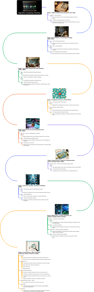
Algorithm complexity is a fundamental concept that quantifies the resources required by algorithms, shaping the landscape of computation from ancient times to the modern era. This overview outlines its evolution across nine stages 1. Origins of measurement (Pre-1900) with Euclid’s algorithm. 2. Formal models of computation emerging (1900–1950s) through Gödel and Turing. 3. Asymptotic analysis standardizing in the 1950s–60s with Big-O notation. 4. Complexity theory solidifying as a field in the 1970s, highlighted by Cook’s theorem. 5. Practical implications in cryptography and randomized algorithms (1970s–80s). 6. Approximation and parameterized complexity (1990s). 7. New cost models and data scale considerations (2000s). 8. The modern era addressing machine learning and quantum complexity (2010s–Present). 9. A timeless definition encompassing the essence of algorithm complexity.
Edited at 2026-03-24 12:39:23
- 小紅書(RED)草もみ転換パス分析図
小紅書(RED)における「草もみ」から購買への転換パスを徹底分析しました。まず、コンテンツの露出や認知段階に焦点を当て、最適な露出チャネルやアルゴリズム推薦の重要性を探ります。続いて、ユーザーの関与を促進する要素や、コメントやQ&Aによる信頼構築について考察。購買段階では、シームレスな決済体験や主要決済手段との連携が鍵となります。最後に、購入後のUGC生成やハッシュタグキャンペーンによるブランド資産の構築についても触れます
- Naver Shopping転換ファネル分析図
Naver Shoppingの転換ファネル分析図は、顧客の購買プロセスを深く理解するための重要なツールです。まず、流入・集客フェーズでは、検索トラフィックやコンテンツディスカバリーを通じてユーザーを引き寄せます。次に、関心・検討フェーズでは、コンテンツとコマースの融合を活用し、情報比較を促進します。意思決定・転換フェーズでは、購入障壁の除去や決済の利便性を重視し、リピート購入を促進する保持・拡散フェーズでは、ユーザー生成コンテンツの循環を通じて新たな顧客を引き込む仕組みを構築しています
- WooCommerce転換パス最適化図
WooCommerceの転換パス最適化は、オンラインストアの成長を促進するための重要な戦略です。このプロセスは、集客からリテンションまでの各フェーズにおいて、効果的な施策を展開します。まず、集客・流入フェーズでは、SEOや有料広告を活用し、ランディングページの最適化を行います。次に、閲覧・検討フェーズでは、商品ページの改善と社会的証明を強調します。カート投入フェーズでは、放棄率を抑制し、決済・チェックアウトフェーズでは簡素化を図ります。購入完了後は、リテンション施策を通じて顧客を再度呼び戻し、データ分析を通じて継続的な改善を実施します
What is Boolean Algebra
- 小紅書(RED)草もみ転換パス分析図
小紅書(RED)における「草もみ」から購買への転換パスを徹底分析しました。まず、コンテンツの露出や認知段階に焦点を当て、最適な露出チャネルやアルゴリズム推薦の重要性を探ります。続いて、ユーザーの関与を促進する要素や、コメントやQ&Aによる信頼構築について考察。購買段階では、シームレスな決済体験や主要決済手段との連携が鍵となります。最後に、購入後のUGC生成やハッシュタグキャンペーンによるブランド資産の構築についても触れます
- Naver Shopping転換ファネル分析図
Naver Shoppingの転換ファネル分析図は、顧客の購買プロセスを深く理解するための重要なツールです。まず、流入・集客フェーズでは、検索トラフィックやコンテンツディスカバリーを通じてユーザーを引き寄せます。次に、関心・検討フェーズでは、コンテンツとコマースの融合を活用し、情報比較を促進します。意思決定・転換フェーズでは、購入障壁の除去や決済の利便性を重視し、リピート購入を促進する保持・拡散フェーズでは、ユーザー生成コンテンツの循環を通じて新たな顧客を引き込む仕組みを構築しています
- WooCommerce転換パス最適化図
WooCommerceの転換パス最適化は、オンラインストアの成長を促進するための重要な戦略です。このプロセスは、集客からリテンションまでの各フェーズにおいて、効果的な施策を展開します。まず、集客・流入フェーズでは、SEOや有料広告を活用し、ランディングページの最適化を行います。次に、閲覧・検討フェーズでは、商品ページの改善と社会的証明を強調します。カート投入フェーズでは、放棄率を抑制し、決済・チェックアウトフェーズでは簡素化を図ります。購入完了後は、リテンション施策を通じて顧客を再度呼び戻し、データ分析を通じて継続的な改善を実施します
- Recommended to you
- Outline