MindMap Gallery What is Algorithm Complexity
Explore the fascinating evolution of algorithm complexity, a concept that underpins the efficiency of computation. This journey begins with early algorithms in ancient times and transitions through key developments in formal models, asymptotic analysis, and complexity theory. Discover the impact of computational challenges in cryptography, the rise of approximation techniques, and modern considerations of data scale and machine learning. The narrative culminates in a timeless definition of algorithm complexity, highlighting its significance in understanding resource requirements for computation across various contexts. Join us in tracing this crucial aspect of computer science!
Edited at 2026-03-24 12:39:26小紅書(RED)における「草もみ」から購買への転換パスを徹底分析しました。まず、コンテンツの露出や認知段階に焦点を当て、最適な露出チャネルやアルゴリズム推薦の重要性を探ります。続いて、ユーザーの関与を促進する要素や、コメントやQ&Aによる信頼構築について考察。購買段階では、シームレスな決済体験や主要決済手段との連携が鍵となります。最後に、購入後のUGC生成やハッシュタグキャンペーンによるブランド資産の構築についても触れます

Naver Shoppingの転換ファネル分析図は、顧客の購買プロセスを深く理解するための重要なツールです。まず、流入・集客フェーズでは、検索トラフィックやコンテンツディスカバリーを通じてユーザーを引き寄せます。次に、関心・検討フェーズでは、コンテンツとコマースの融合を活用し、情報比較を促進します。意思決定・転換フェーズでは、購入障壁の除去や決済の利便性を重視し、リピート購入を促進する保持・拡散フェーズでは、ユーザー生成コンテンツの循環を通じて新たな顧客を引き込む仕組みを構築しています
WooCommerceの転換パス最適化は、オンラインストアの成長を促進するための重要な戦略です。このプロセスは、集客からリテンションまでの各フェーズにおいて、効果的な施策を展開します。まず、集客・流入フェーズでは、SEOや有料広告を活用し、ランディングページの最適化を行います。次に、閲覧・検討フェーズでは、商品ページの改善と社会的証明を強調します。カート投入フェーズでは、放棄率を抑制し、決済・チェックアウトフェーズでは簡素化を図ります。購入完了後は、リテンション施策を通じて顧客を再度呼び戻し、データ分析を通じて継続的な改善を実施します
小紅書(RED)における「草もみ」から購買への転換パスを徹底分析しました。まず、コンテンツの露出や認知段階に焦点を当て、最適な露出チャネルやアルゴリズム推薦の重要性を探ります。続いて、ユーザーの関与を促進する要素や、コメントやQ&Aによる信頼構築について考察。購買段階では、シームレスな決済体験や主要決済手段との連携が鍵となります。最後に、購入後のUGC生成やハッシュタグキャンペーンによるブランド資産の構築についても触れます
Naver Shoppingの転換ファネル分析図は、顧客の購買プロセスを深く理解するための重要なツールです。まず、流入・集客フェーズでは、検索トラフィックやコンテンツディスカバリーを通じてユーザーを引き寄せます。次に、関心・検討フェーズでは、コンテンツとコマースの融合を活用し、情報比較を促進します。意思決定・転換フェーズでは、購入障壁の除去や決済の利便性を重視し、リピート購入を促進する保持・拡散フェーズでは、ユーザー生成コンテンツの循環を通じて新たな顧客を引き込む仕組みを構築しています
WooCommerceの転換パス最適化は、オンラインストアの成長を促進するための重要な戦略です。このプロセスは、集客からリテンションまでの各フェーズにおいて、効果的な施策を展開します。まず、集客・流入フェーズでは、SEOや有料広告を活用し、ランディングページの最適化を行います。次に、閲覧・検討フェーズでは、商品ページの改善と社会的証明を強調します。カート投入フェーズでは、放棄率を抑制し、決済・チェックアウトフェーズでは簡素化を図ります。購入完了後は、リテンション施策を通じて顧客を再度呼び戻し、データ分析を通じて継続的な改善を実施します
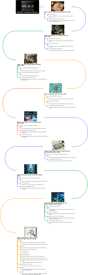
Algorithm Complexity (Timeline)
Stage 1: Origins of Measuring Computation (Pre-1900)
c. 300 BCE — Euclid’s algorithm
Early known algorithm; raises “how many steps” depends on input size
1800s — Growth of mathematical analysis of procedures
Number theory/analysis informally studies computational effort (e.g., Gauss), not yet formal complexity theory
Stage 2: Formal Models of Computation Emerge (1900–1950s)
1931 — Gödel’s incompleteness theorems
Motivates formal reasoning about what can be computed/proven within a system
1936 — Church–Turing foundations
λ-calculus and Turing machines enable precise definitions of time/space as resources
1940s — Early programming and cost awareness
Real constraints (memory, CPU time) push systematic performance analysis
Stage 3: Asymptotic Analysis Becomes Standard (1950s–1960s)
1950s — Big-O notation popularized in algorithm analysis
Big-O/Ω/Θ become standard for growth rates as input size n increases
1959 — Cobham’s characterization of feasible computation
Links “efficiently computable” with polynomial time
1960s — Algorithm design and analysis matures
Sorting/searching/graph algorithms analyzed for worst/average time; space becomes formal
Stage 4: Complexity Theory as a Field (1970s)
1971 — Cook’s theorem (SAT is NP-complete)
Establishes NP-completeness and reductions; “hardness” becomes central
1972 — Karp’s NP-complete problems
Many important problems shown NP-complete; major practical relevance
1970s — Complexity classes formalized and studied
P, NP, co-NP, PSPACE; completeness, reductions, hierarchies become standard toolkit
Stage 5: Practical Impact and Cryptography (Late 1970s–1980s)
1976–1978 — Public-key cryptography and complexity
RSA and related schemes rely on hardness assumptions (e.g., factoring)
1980s — Randomization and probabilistic classes
Randomized algorithms; BPP/RP; expected time and error probability enter complexity
1980s — Average-case vs worst-case
Separates worst-case hardness from typical performance; motivates average-case complexity
Stage 6: Approximation, Hardness of Approximation, and Fine-Grained Views (1990s)
Early–mid 1990s — PCP theorem and hardness of approximation
Limits approximability unless P=NP; links verification structure to approximation
1990s — Parameterized complexity develops
Complexity in terms of n and parameter k; FPT vs W[1]-hardness lens
Stage 7: Data Scale, Systems, and New Cost Models (2000s)
2000s — External-memory and cache-aware/oblivious models
Measures I/O operations and cache misses; bottlenecks beyond CPU steps
2000s — Streaming algorithms
Passes, memory footprint, update time for massive data streams
2000s — Distributed and parallel complexity
Work/span, communication complexity, network models for large-scale computation
Stage 8: Modern Era—Learning, Quantum, and Hardware Realities (2010s–Present)
2010s — Complexity in machine learning
Training/inference cost, sample complexity, optimization complexity; accuracy vs budget tradeoffs
2010s — Fine-grained complexity
Precise bounds (near-quadratic vs near-linear); conditional lower bounds (e.g., SETH)
2010s–2020s — Quantum complexity and algorithms
Quantum models (BQP, etc.) and algorithms (simulation, factoring) reshape “efficient” under new hardware
2020s — Energy and carbon-aware computation
Energy complexity complements time/space as real-world constraints
Stage 9: Core Definition—What “Algorithm Complexity” Means (Timeless Concept)
Definition
Describes how required computational resources grow with input size n
Main resources: time complexity (operations) and space complexity (memory)
Asymptotic focus
Uses growth-rate notation to ignore constants/lower-order terms for large n
Big-O: upper bound (worst-case growth rate)
Big-Ω: lower bound
Big-Θ: tight bound
Common analysis perspectives
Worst-case complexity: maximum resources over all inputs of size n
Average-case complexity: expected resources under an input distribution
Amortized complexity: average per operation over a sequence (e.g., dynamic arrays)
Expected complexity: expectation over algorithm randomness
Typical growth rates (smaller → larger)
O(1), O(log n), O(n), O(n log n), O(n²), O(n³), O(2ⁿ), O(n!)
Why it matters
Predicts scalability, guides algorithm choice/design, explains feasibility (polynomial vs exponential)
Key caveats
Asymptotics can hide large constants; performance depends on hardware, memory hierarchy, input structure, implementation details