Features
Features:

Product Tour >

Edraw AI >

Paid Plans:

Individuals >

Business >

Eduaction >
Resources
Blog

History

How-tos & Tips

Discovery

Biography

Business Analysis

Examples

AI concept Map

Free AI Mind Map Generator

Onenote Mind Map

Bcg Matrix Examples

Nike Marketing Strategy

Unilever SWOT Analysis

Make Mind Maps in Google Docs

Guide

FAQs

What's New

Resource Center
Templates
All Templates

Brain Storming Templates

Strategy and Planning Templates

Project Management Templates

Product Management Templates

Human Resources Templates

Agile Workflow Templates

Marketing Templates

Education Templates

Fun and Games Templates

User Gallery
Download
Pricing
Enterprise

MindMap Gallery Machine learning algorithm linear regression decision tree notes self-study mind map

Machine learning algorithm linear regression decision tree notes self-study mind map

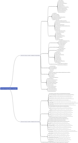
Machine learning algorithm linear regression decision number notes self-study complete sharing! The content covers K-nearest neighbor algorithm, linear regression, logistic regression, decision tree, ensemble learning and clustering.

Edited at 2023-02-25 09:44:36

PlotWizard

Recent works View more works>>

Machine learning algorithm linear regression decision tree notes self-study mind map

PlotWizard

Recent works View more works>>

Recommended to you
Outline

Bivariate statistical measurement
- 53
- 1
Claudia Galeano
Machine learning algorithm classification
- 59
PlotWizard
Top 10 algorithms in artificial intelligence
- 59
PlotWizard
Decision tree architecture algorithm programming mind map
- 53
PlotWizard
Basic regression algorithm for machine learning
- 38
PlotWizard
linear regression
- 55
Gavinnblake
Machine learning algorithm and nomogram construction for prediction of diabetic retinopathy in patients with type 2 diabetes
- 14
Gavinnblake
Monday Decision Tree
- 8
MMzVlzoz

Machine learning algorithm linear regression decision tree notes self-study mind map

K-nearest neighbor algorithm

Algorithm principles and API

The concept and principle of K-nearest neighbor algorithm

concept

If most of the k most similar (i.e. nearest neighbors in feature space) samples of a sample belong to a certain category, then the sample also belongs to this category.

feature space

A space established using all features as coordinate axes. In the feature space, each sample is a point.

[Key points] Principle and implementation steps

1. Calculate the distance between the point in the known category data set and the current point

2. Arrange these distances in ascending order

3. Select the k points with the smallest distance from the current point

4. Count the frequency of occurrence of the category where the first k points are located (find the mode of the K categories)

5. Use the mode category as the category of the current point

K-Nearest Neighbor Algorithm API

Introduction to Scikit-learn

Machine learning tools that implement numerous machine learning algorithms

API

sklearn.neighbors.KNeighborsclassfier(n_neighbors)

Algorithm calculation and optimization

measure of distance

Euclidean distance

Manhattan distance (block distance)

Chebyshev distance

Minkowski distance (Min's distance)

Normalized Euclidean distance

cosine distance

Hamming distance

String lengths are equal

Calculate distance of string

Jaccard distance

distance between two sets

Mahalanobis distance

The impact of the choice of K value on the model

Performance of underfitting and overfitting

approximation error

The error of the model on the training set

estimation error

The error of the model on the test set

Underfitting

The approximation error is large and the estimation error is large. To put it bluntly, the model performs poorly on both the training set and the test set.

overfitting

The approximation error is small, but the estimation error is large. To put it bluntly, the model performs well on the training set but not on the test set.

K value is too small

Largely affected by outliers

The model is complex, has strong learning ability, and is prone to overfitting.

K value is too large

The impact of sample imbalance is large

The model is simple, has weak learning ability, and is prone to underfitting.

kd tree

kd tree introduction

tree concept

root node

Nodes with only child nodes and no parent nodes

internal node

Nodes that have child nodes and parent nodes

leaf node

Nodes with only parent nodes and no child nodes

Binary tree

A tree with at most two forked nodes

The role of kd tree

Reduce the number of calculations of sample distance and quickly find the nearest neighbor point

Construction method of kd tree

1. Randomly select a feature, take the median of this feature as the dividing point to divide the data into two equal parts. The selected feature is the dividing feature of the current node, and the median point is used as the current node. On this feature, points smaller than the median are classified into the left node, and points larger than the median are classified into the right node;

2. Repeat the first step for the data on the left node and the right node respectively;

3. Until all samples are placed on the node

How to find the nearest point in kd tree

1. Compare the query point M with the dividing characteristics and corresponding median of each node on the kd tree, and continue to compare downward until reaching the leaf node. Record in order the nodes traveled through the entire process search_path;

2. The node at the end of search_path is N, do not take out N, record the distance between dist=M and N, nearest=N;

3. Take out a node L from the end of search_path, the dividing axis of this node is x, calculate the distance a from point M to the x axis, and then handle it in two cases:

If a<dist, then all points in the space on the other side divided by node L and the current nearest point are included in the investigation range, the distances from all points in the investigation range to point M are calculated, the nearest point is found, and the point is recorded as nearest. The distance from this point to M is dist, discard node L, and the step ends;

If a>=dist, discard node L and the step ends

4. Repeat step 3 until search_path is empty;

5. Nearest is the point closest to the search point, and the nearest distance is dist.

Case 1

Introduction to the dataset API of scikit-learn

sklearn small data set

API: load_* Such as: load_iris()

sklearn big data set

API: fetch_* Such as: fetch_20newsgroups(sub_set='train')

Parameter description: sub_set='train' specifies the type of data set to be obtained

Introduction to sklearn data set return value

Data type: datasets.base.Bunch (dictionary format)

data: feature data array

target: array of labels (target values)

feature_names: feature names

target_names: tag names

keys() gets all attributes (fields) of the dictionary

Draw a scatter plot of data and find outliers

sns.lmplot(col1, col2, data, hue, fit_reg)

Partition of the data set

x_train, x_test, y_train, y_test = trian_test_split(x, y, test_size)

Feature preprocessing using sklearn

Normalized

Disadvantages of normalization: greatly affected by outliers

API: MinMaxScaler(feature_range)

Function: Convert data to between 0 and 1

standardization

API:StandarScalar()

Function: Convert data to mean=0, std=1

Iris flower species prediction

Case 2

Cross-validation and grid search

Cross-validation

Divide the training set evenly into N parts, take a different part as the verification set, and the other part as the training set, train and verify the model performance, and use the average of the N times of model performance as the performance of the model on this training set.

grid search

Find the optimal combination of hyperparameters

API

sklearn.model_selection.GridSearchCV(estimator, param_grid, cv)

Predict Facebook check-in location

linear regression

Introduction to Linear Regression

Mathematical formula (mathematical model) of linear regression

h(w) = w1*x1 w2*x2 w3*x3 ... wn*xn b

The concept of hyperplane

The n-1 dimensional linear relationship in n-dimensional space is called a hyperplane in n-dimensional space.

API

sklearn.linear_model.LinearRegression()

Losses and Optimization for Linear Regression

loss function

1. The loss function is a function of the trainable parameters

2. The smaller the value of the loss function, the closer the model’s predicted value is to the true value.

Optimization method of linear regression

normal equation

Calculate optimal parameters directly

NOTE: Applicable only to linear regression models with least squares loss

gradient descent method

Continuously iterate through gradients to find optimal trainable parameters

General optimization methods

Loss function Gradient descent is the most common model optimization method

gradient descent method

Full Gradient Descent Algorithm (FG)

Stochastic Gradient Descent Algorithm (SG)

Stochastic Average Gradient Descent Algorithm (SAG)

Mini-batch gradient descent algorithm (mini-bantch)

Case-Boston House Price Forecast

Regression performance evaluation API: sklearn.metrics.mean_squared_error(y_true, y_pred)

Normal equation optimization linear regression API: sklearn.linear_model.LinearRegression()

Optimizing linear regression with stochastic gradient descent: sklearn.linear_model.SGDRegressor()

Overfitting and underfitting

Underfitting

Definition: The model performs poorly on both the training set and the test set

Solution: Increase model complexity

Increase the number of features of the data

Add polynomial terms

overfitting

Definition: The model performs well on the training set, but does not perform well on the test set

Solution: Reduce model complexity

Clean the data again

Increase the amount of training data

Regularization

L1 regularization: You can make some of the W values directly 0, removing the influence of this feature. Can be used for feature selection

L2 regularization: It can make some of the W's very small and close to 0, weakening the influence of a certain feature.

Reduce the number of features

regularized linear model

ridge regression

Linear regression L2 regularization

Lasso returns

Linear regression L1 regularization

elastic network

Linear regression L1 L2

ridge regression

Linear regression with L2 regularization

API: Ridge(alpha)

Saving and loading models

Save: joblib.dump(estimator, path)

Loading: joblib.load(path)

logistic regression

The principles of logistic regression

Mathematical model: linear regression activation function (sigmoid)

The role of the activation function: increase the nonlinear fitting ability of the model

Loss function: Log-likelihood loss

Optimization method: gradient descent

API: sklearn.linear_model.LogisticRegression()

How to evaluate classification models

Classification evaluation report API: classification_report(y_true, y_pred, label, target_names)

ROC curve

TPR = TP / (TP FN)

FPR = FP / (FP TN)

Adjust the threshold to obtain multiple (FPR, TPR) points and draw the ROC curve

AUC indicator

Meaning: randomly select a pair of positive and negative samples, the probability that the score of the positive sample is greater than that of the negative sample

API: roc_auc_score(y_true, y_score), note: y_true must use 0, 1 to mark false cases and positive cases

decision tree

Introduction to decision tree algorithm

Decision tree is a tree structure

Each internal node represents the judgment of a feature

Each branch represents the output of a judgment result

Each leaf node represents a classification result

The principle of decision tree

Feature selection and division basis of decision tree nodes

entropy

A measure of “chaos”

entropy = -p1logp1 - p2logp2 ... pn*log(pn)

information gain

The difference in entropy before and after dividing the data set by a certain feature

Information gain = entroy(before) - entroy(after)

The greater the information gain, the better the classification method of this feature.

information gain rate

Information gain/separated information metric

Separation information measure = entropy calculated from the probability of occurrence of each category of a feature

Gini gain

Gini value: The probability that two samples randomly selected from the data set D have inconsistent target values (labels)

The smaller the Gini value, the higher the purity of the data set.

Gini gain = Gini value (before) - Gini value (after)

The greater the Gini value gain, the better this division method is.

Steps to build a decision tree

1. Start looking at all samples as a whole

2. Traverse each segmentation method of each feature and find the best segmentation (based on information gain, information gain rate, and Gini value gain)

3. According to the optimal division method, divide all samples into two parts N1 and N2, that is, two branches

4. Continue steps 2-3 for N1 and N2 until each node is "pure" enough.

According to different node selection and division basis, the decision tree is divided into

ID3 decision tree: information gain

C4.5 Decision Tree: Information Gain Rate

CART decision tree: Gini value gain (or Gini index)

cart pruning

Purpose: Reduce the number of decision tree nodes -> Reduce the complexity of the decision tree -> Prevent the decision tree from overfitting

method

Pre-pruning: Pruning when creating a decision tree

The minimum number of samples contained in each node, such as 10. If the total number of samples at the node is less than 10, no classification will be performed.

Specify the height or depth of the tree, for example, the maximum depth of the tree is 4

If the entropy of the specified node is less than a certain value, it will no longer be divided.

Post-pruning: pruning after creating the decision tree

The method is similar to pre-pruning

Feature Engineering: Feature Extraction

Dictionary feature extraction

sklearn.feature_extraction.DictVectorizer(sparse=True)

Note: This method will automatically one_hot encode discrete data

Text feature extraction

word occurrence count

sklearn.feature_extraction.text.CountVectorizer(stop_words=[])

Tf-idf text feature extraction

TF: word frequency

Refers to the frequency of a given word appearing in the document

IDF: inverse document frequency

Divide the total number of documents by the number of documents containing the word, and then take the base 10 logarithm of the quotient to get

TF-IDF

TF-IDF = TF*IDF

Function: Evaluate the importance of a word to a document set or a document in a corpus

API:sklearn.feature_extraction.text.TfidfVectorizer(stop_works)

Note: To extract features from Chinese articles, word segmentation must be performed first.

Stuttering participle: jieba.cut

Case: Titanic passenger survival prediction

Decision tree API: sklearn.tree.DecisionTreeClassifier(criterion=’gini’, max_depth=None,random_state=None)

Decision tree visualization: sklearn.tree.export_graphviz()

Summarize

Advantages of decision trees: simple, interpretable, and visualizable

Disadvantages of decision trees: easy to overfit

Solution

pruning

random forest

Ensemble learning

Introduction to ensemble learning algorithms

Generate multiple classifiers/models, each learning and making predictions independently. These predictions are ultimately combined into a combined prediction that is better than any single classification prediction.

boosting -> underfitting

bagging -> overfitting

Bagging ensemble learning

Principle: Build multiple models in parallel, and the models are independent of each other

1. Sampling: Sampling N pieces of data with random replacement

2. Learning: Use N pieces of data to learn N different models

3. Integration: Through equal voting of N models, the one with the most votes will be the final result.

random forest

What is random forest: bagging decision tree

API:sklearn.ensemble.RandomForestClassifier(n_estimators, max_depth)

advantage

Both methods can improve the generalization accuracy rate by about 2% on the original algorithm.

Simple, convenient and versatile

Boosting integration principle: Build multiple models in series, and the model built later is affected by the model built previously.

1. Initialize the training weights, make the weights equal, and train the first learner (model)

2. Calculate the error rate of the learner in the training data

3. Calculate the weight of the learner based on the error rate

4. Reweight the training data according to the weight of the learner

5. Repeat steps 1~4 m times

6. Weighted voting on the results of m models to obtain the final result

clustering

Introduction to clustering algorithms

Clustering algorithm is a typical unsupervised learning algorithm, mainly used to automatically classify similar samples into a category

The biggest difference between clustering algorithms and classification algorithms: clustering algorithms are unsupervised learning algorithms, and classification algorithms are supervised learning algorithms.

Initial use of clustering algorithm API

sklearn.cluster.KMeans(n_clusters=8)

Prediction method: Call fit_predict(X) to get the classification results

Clustering algorithm implementation process (principle)

1. Randomly select K samples as the centers of K categories;

2. Calculate the distance from all samples to the center;

3. Which category the sample is closest to the center;

4. After dividing K categories, recalculate the coordinates of the center. The calculation method is that the average value of each feature value of the samples in the category is used as the corresponding coordinates of the new center;

5. Repeat steps 2, 3, and 4 until the coordinates of the center no longer change.

Model evaluation for clustering

Sum of squared errors: the sum of the squared distances (Euclidean distance) of all samples to the corresponding category center

"Elbow" method: when the decline rate suddenly slows down, it is considered to be the best k value

SC silhouette coefficient: The value is [-1, 1]. The larger the value, the better. If it is a negative value, the sample may be classified incorrectly.

CH coefficient: The higher the score s, the better the clustering effect.

Algorithm optimization

Canopy algorithm with initial clustering

K-means

Bipartite k-means

ISODATA

kernel kmeans

Mini-batch K-Means

Feature dimensionality reduction

Feature selection

Remove low variance features

Pearson correlation coefficient

Spearman correlation coefficient

Principal Component Analysis PCA

Case: Exploring user preferences for item categories and dimensionality reduction